Applied Mathematics
Vol.06 No.11(2015), Article ID:60339,21 pages
10.4236/am.2015.611160
Unique Measure for the Time-Periodic Navier-Stokes on the Sphere
Gregory Varner
Division of Natural and Health Sciences, Mathematics Department, John Brown University, Siloam Springs, USA
Email: gvarner@jbu.edu
Copyright © 2015 by author and Scientific Research Publishing Inc.
This work is licensed under the Creative Commons Attribution International License (CC BY).
http://creativecommons.org/licenses/by/4.0/


Received 2 September 2015; accepted 13 October 2015; published 16 October 2015
ABSTRACT
This paper proves the existence and uniqueness of a time-invariant measure for the 2D Navier- Stokes equations on the sphere under a random kick-force and a time-periodic deterministic force. Several examples of deterministic force satisfying the necessary conditions for a unique invariant measure to exist are given. The support of the measure is examined and given explicitly for several cases.
Keywords:
Navier-Stokes, Invariant Measure, Sphere

1. Introduction
The existence and uniqueness of a time-invariant measure for the Navier-Stokes equations has been the subject of much recent research. A major advance was achieved in [1] where it was shown that, under a random bounded kick-type force, the Navier-Stokes system on the torus (bounded domains with smooth boundaries and periodic boundary conditions) has a unique time-invariant measure. Subsequently, the argument was refined to a more flexible coupling approach in [2] , which paved the way for extending the argument to the case of a white-noise random force [3] -[5] . Unfortunately, these methods focused on the equations on the torus and, with the exception of the white-noise random force, the case of zero deterministic forcing on the system. Of course, for meteorological purposes, it is desirable to consider the equations on the sphere and to require the deterministic force to be nonzero. This was done in [6] , where a time-invariant measure for the Navier-Stokes equations on the sphere was shown to exist both under a random bounded kick-type force with a time-independent deterministic force and under a white-noise force.
This paper extends the work in [6] to include time-periodic deterministic forces. A similar result was established in [7] for the torus and with a random perturbation activated by an indicator function. Even though the random force in [7] allowed more general time-dependence, stronger assumptions on the regularity of both the random force and the deterministic force are needed. We instead use a random perturbation activated by a Dirac function as in [2] [6] to allow a broader class of random and deterministic forces through weaker regularity assumptions and to highlight the similarities between the time-independent and time-periodic cases. Furthermore, the more general case of a squeezing-type property of the deterministic equations is included, allowing for more general time-periodic deterministic forces.
The first section uses a combination of the approaches in [8] -[11] to define each of the terms in the Navier- Stokes equations on the sphere. Of utmost importance are the eigenvalues of the Laplacian term which allow the analysis to proceed as in the case of flat domains. In addition, we consider the Navier-Stokes equations under time-periodic forcing, establishing conditions for there to be a limiting solution that is periodic. By extending results in [6] , several cases are considered where the period of the unique solution is the same as the force. In particular, if a solution has only latitudinal dependence or is very “close” to having only latitudinal dependence then the solution is unique with the same period as the force.
The second section presents the main theorem, which establishes the existence and uniqueness of an invariant measure for the kicked equations with a time-periodic deterministic external force. The proof of the main theorem is done by proving that necessary conditions hold for the applicability of Theorem 3.2.5 in [12] . As will be seen, the periodicity of the deterministic force allows the argument for stationary forces to be applied to the time-periodic case. The necessary conditions for the main theorem are shown for several cases including a contraction-type property and a squeezing-type property with “large” random kicks. The main idea behind the contraction-type property is the exponential stability of solutions, i.e., the contraction of the flow to a unique solution, while the squeezing-type property is related to the idea of determining modes ([13] , p. 363) and generalizes the concept of a finitely stable point introduced by the author in [6] . More precisely, if the projection of the initial conditions onto the first M eigenfunctions is close enough then the solutions will converge.
The third section recalls work done by the author in [6] describing the support of the measure. The support is described both in general and specifically for several examples. By combining results in [6] [14] , the support of the measure is described in terms of a unique time-periodic solution in several cases, including some of potential meteorological interest.
2. The Navier-Stokes Equations on the Sphere
Let  be the 2-dimensional sphere with the Riemannian metric induced from R3. Let
  be the spherical coordinate system on M, where
  is the co-latitude (the geographical latitude) and
  is the longitude, and, thus,
  is the outward normal to M in R3. Let
  and
and , then the unit vectors

form a basis for the tangent space of M, denoted TM, and induce on M the Reimannian metric

The Navier-Stokes equations on the rotating sphere are
 (1)
(1)
where n is the normal vector to the sphere,  is the Coriolis coefficient,
  is the angular velocity of the Earth, and “´” is the standard cross product in
 .
.
The operators  and
and  in (1) have their conventional meanings on the sphere, i.e. for functions
  and vectors u

where .
.
To define the covariant derivative  and the vector Laplacian ∆ we first define the curl of a vector in terms of extensions. For any covering
  of M by open sets, there is a corresponding set of “cylindrical domains”
  that cover a tubular neighborhood of M,
 . In each
  introduce the orthogonal coordinate system
 , where
  is along the normal to M and for
  the coordinates
  agree with the spherical coordinates.
For a vector  there is a vector
  defined in
  such that the restriction to M satisfies
  . For a vector field w on the sphere, not necessarily tangent to it, the curl of w is a vector field along the sphere defined as ([9] , p. 562)
For a vector field normal to M, the curl is well-defined and is tangent to M. However, for a vector field in TM the curl is not well-defined but the third component of the curl, denoted curln, is well-defined. Due to this, define the following operators ([11] , p. 344).
Definition 1. Let u be a smooth vector field on M with values in TM and let  be a smooth vector field on M with values in
 , i.e.
  for
for  a smooth scalar function (thus we identify
  with the function
 ). Denote the extensions
  and
and . Then for
 ,
,  define


where on the right side Curl denotes the standard curl operator in  and these definitions are independent of the extensions ([9] , p. 562).
The covariant derivative and vector Laplacian are now defined in terms of the curl and curln operators ([9] , p. 562-563).
Definition 2. The covariant derivative on the sphere is given by
 (2)
(2)
Remark 3. As with the curl and curln operators, it is possible to define the gradient, divergence, and covariant derivative in terms of extensions (see [8] [9] ). However ([11] , p. 344),

Thus both curl and curln, and thus the gradient, divergence, and covariant derivative, can be defined without resorting to extensions.
Definition 4. The vector Laplacian on the sphere is given by ([9] , p. 563)
 (3)
(3)
Thus, the Navier-Stokes equations on the two-dimensional sphere, i.e., for vector fields on M, are:
 (4)
(4)
2.1. Existence and Uniqueness for the Deterministic Equations
Let  and
and  be the standard
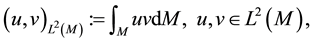
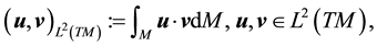
  -spaces of the square integrable scalar functions and tangent vector fields on M, respectively. The inner products for
  and
and  are given by:
with the induced norm on  denoted
 . Note that these are integrals over oriented manifolds and thus are defined intrinsically using a partition of unity. Locally, however,
 .
.
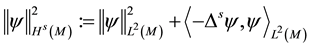
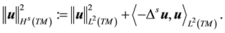
Let  be a scalar function and v be a vector field on M. For
 , the standard Sobolev spaces Hs have norm
and
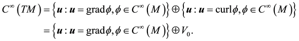
By the Hodge Decomposition Theorem, the space of smooth vector fields on M can be decomposed as ([9] , p. 564):
Define the following closed subspaces of  and
and  respectively:
Definition 5.

with norm
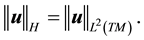 (5)
(5)
Note, H is the L2 closure of V0 and thus  for
for .
.
Definition 6.
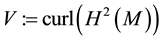
with norm
 (6)
(6)
Note, V is the H1 closure of V0 and thus  for
for . Furthermore, V is compactly embedded into H, and by the Poincare Inequality (Equation (41)) the V norm is equivalent to the H1 norm for divergence-free vector fields.
Definition 7. For a vector field u, define the Laplacian on divergence-free vector fields as
 (7)
(7)
Furthermore, if  then
then .
.
The following theorem implies that the analysis used for the stochastic Navier-Stokes system on flat domains can be used for the system on the sphere. Its proof is identical to the case of flat domains with smooth boundary conditions, see [13] , pp. 162-163 or [9] , p. 565.
Theorem 8. The operator  is a self-adjoint positive-definite operator in H with eigenvalues
  with the only accumulation point
 . Moreover, the eigenvalues correspond to an orthonormal basis in H (orthogonal in V).
Let  be the projection onto H. Since the projection commutes with
  and A, the projection of the Navier-Stokes equations onto H is
 (8)
(8)
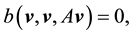
where . Furthermore, for all
 (9)
(9)
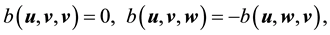
where  is the standard trilinear form associated with the Navier-Stokes equations, i.e.
 (10)
(10)
where  is the orthogonal projection onto TM ([9] , p. 561), and the trilinear terms satisfies estimates analogous to those in the case of flat domains, see Lemma 12.
We now state the existence and uniqueness of solutions to the deterministic Navier-Stokes equations in terms of the projected equations, as is standard.
Theorem 9. Suppose  and
and  then a solution of Equation (8) exists uniquely and
 . If
. If  then the solution is strong, i.e.
and .
.
The proof is the same as the case of bounded domains with smooth boundaries and periodic boundary conditions (see [13] , pp. 245-254 and [9] , Theorem 2.2).
2.2. Time-Periodic Navier-Stokes Equations on the Sphere
Let the deterministic force  (thus
(thus  for any
 ) be periodic with period T > 0. While Theorem 9 gives the existence of a strong solution to the Navier-Stokes equations on the sphere, it will be necessary to know the behavior of the system under a periodic force. Toward that end, we recall a theorem from [14] , p. 19.
Definition 10. Let  be a perturbation of the solution u of the Navier-Stokes equations. u is exponentially stable if there exist numbers
  such that every perturbation at time
 , with
  and
and  satisfies
 (11)
(11)
 is called the stability radius.
Theorem 11. Suppose there exists a globally defined solution to the Navier-Stokes equation with initial condition in H, has  bounded, and is exponentially stable. If f is time-periodic with period T then there exists a time-periodic solution
  with period kT for some integer k, such that
 (12)
(12)
If the stability radius δ is large enough or the period is small enough then . In all cases,
  is exponentially stable.
While the theorem in [14] assumes that the initial condition is in H1, this is for  to be bounded. By Theorem 9 (or Equation (55)) this norm is bounded for
  and any t > 0. Furthermore, Theorem 11 implies convergence in H and the proof in [14] is easily adapted to show exponential convergence in H instead.
It is well-known that if the force is small enough (see Remark 33) then the stability radius is infinite and thus there is a unique exponentially stable solution with the same period as the force that all other solutions converge to. We conclude this section by examining two more cases where the stability radius is infinite. The proofs of the following lemmas are found in the Appendix. The main idea behind both of the lemmas is that the (spherical) scalar Laplacian commutes with longitudinal derivatives, allowing for terms in the calculations only dependent on latitude to vanish.
Definition 12. A solution to the Navier-Stokes equations, u, is called zonal if for each fixed t,  is only a function of latitude, i.e. the function has no longitudinal dependence.
Lemma 1. Suppose that the time-periodic force  is such that there is a zonal solution. Then the solution is unique with the same period as f.
Remark 13. For a stationary force, it is sufficient that the force is zonal to have a stationary zonal solution ([10] , p. 988) which follows since A forms an isomorphism between the spaces  and H and for u zonal

Analogously, the Stoke’s equation  forms an isomorphism between the spaces

Thus, to have a zonal solution it is sufficient that force is zonal. (The proof that the equations form an isomorphism is analogous to the result in [15] , Lemma 3.1, p. 27 or [16] , Chapter 4, Section 15.)
Lemma 2. Suppose that  is a force that generates a zonal solution. Then there exists
  such that for any force
  such that
  there is a unique globally exponentially stable solution to the Navier-Stokes equations.
Definition 14. We define an almost zonal solution to be a solution guaranteed by Lemma 2.
It is worth noting that while Lemma 2 allows for nonzonal solutions, they are only a “small” perturbation from being zonal.
3. The Main Theorem
This section presents the main theorem on the existence and uniqueness of a (time-)invariant measure for the Navier-Stokes system with random kicks and a time-periodic deterministic force, where time-invariance is understood to mean that the random variables generated by restricting the solutions to instants of time proportional to the period of the deterministic forcing term have a unique stationary probability distribution which all other distributions converge to exponentially (i.e. it is exponentially mixing). A similar result in [7] established that the Navier-Stokes equations on the torus have a unique invariant measure under a deterministic time-periodic forcing. While the random force considered in [7] allows for more generality in the sense of time-dependence, the random force and the deterministic force require more regularity than will be assumed in this paper. Instead we use a bounded random kick-force as in [2] [6] to allow for a larger class of deterministic forces through weaker regularity assumptions and to highlight similarities to the time-independent case which are not as evident in [7] . In particular, we use a modified version of Theorem 3.2.5 in [12] which focuses on the properties of the solution operator and the perturbed flow, which are used more implicitly [7] . In addition, we consider cases of potential meteorological interest and more general deterministic forces than allowed in [7] .
3.1. The Perturbed Navier-Stokes Equations
Consider the Navier-Stokes system with forcing 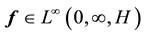 time-periodic with period T, and a random kick-force g bounded in H:
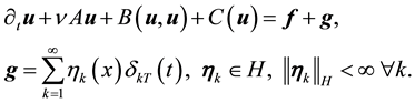 (13)
(13)
The notation from now on will be:
・  is the solution of the deterministic equation with initial condition
  at time
 .
.
・ For simplicity of notation take the period as  and denote
 .
.
・  is the solution of (13) with initial condition
  at time
 .
.
Then
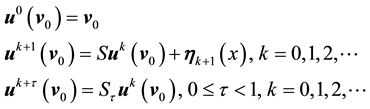 (14)
(14)
In other words, the solution between kicks is given by the flow of the deterministic system with time-periodic forcing. Notice that due to the periodicity of the force, if all the kicks were zero then for any positive integer n, 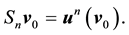
Following [2] , pp. 356-357, assume the kicks satisfy:
Condition 15. Let  be the orthonormal basis for the Hilbert space H, then
 (15)
(15)
for  a family of independent, identically distributed real-valued variables, with
  for all
 . Their common law has density
  with respect to Lebesgue measure where
  is of bounded variation with
support in the interval . Furthermore, for any
 ,
, 
For a given positive integer k and , the Markov transition measure
  is defined as

where  is the Borel
  -algebra of H. The Markov transition measure is the probability that the stochastic flow with initial condition
  is in the set
  at time k, i.e.
 .
.
The Markov semigroup  on bounded continuous functions is defined by
where  is a bounded continuous function.
Definition 16. A measure  is called invariant if
  where
where  is the space of probability measures on H and

The next two definitions deal with behavior of the deterministic flow and are necessary for the statement of the main theorem.
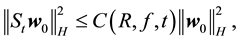
Definition 17. We say that there is an asymptotically stable solution if for some , for all
 , and for all
 (16)
(16)
where  can depend on the norm of the force and
  is the ball of radius R centered at 0 in H.
Notice that an asymptotically stable solution is exponentially stable for any radius .
.
At minimum the following satisfy condition (16):
・  and “small” forces, see Remark 33.
・ Time-periodic forces that give zonal flow, see Lemma 1.
・ Time-periodic forces that give almost zonal flow, see Lemma 2.
While both zonal and almost zonal flow are of potential meteorological interest, Condition (16) is actually restrictive since it guarantees that the exponentially stable solution is unique and that all other solutions converge to it exponentially. Thus it is of interest to consider more general deterministic forces than just the ones that satisfy Condition (16).
Note that since the Navier-Stokes equations have an absorbing set ([9] , p. 572) any asymptotically stable solution is in a ball of finite radius in H, call it  (see Equation (19)). In addition, an asymptotically stable solution guarantees that two deterministic solutions with different initial conditions will become arbitrarily close together as
 . In the same way, any point that locally acts like an asymptotically stable solution will be a (local) contraction of the flow and should be considered. However, since it will be sufficient for the random perturbations to be finite-dimensional (see Theorem 20), it will be sufficient for the solution to be locally stable in a finite number of dimensions.
Definition 18. Let  be the radius of the deterministic absorbing set (i.e. as in Equation (19)) and
  be the projection onto the first M eigenfunctions. A point
  is called finitely stable if for some
 , for some
 , for any
  and for all
  satisfying
 ,
,
 (17)
(17)
In other words, if the finite-dimensional projections are “close enough”, then the solutions converge.
A finitely stable point captures the same concept as determining modes ([13] , page 363) and satisfies the conditions of Theorem 11 (the stability radius and δ from Definition 18 can be taken the same). Furthermore, if δ is large enough relative to T then the periodic solution converged to has period T.
While the assumption of a finitely stable point allows for the possibility of multiple solutions, the assumption also has the disadvantage that we will need additional assumptions on the structure of the kicks.
Definition 19. The following is called the big kick assumption. Let M be as in Definition 18. For some  let the
  from Condition 15 satisfy
 (18)
(18)
where  is the same as in (19) and
  is the eigenvalue corresponding to
 .
.
By Equations (54) and (41) the  are assumed to be twice as large as
  if the initial condition is zero (where
 ). Thus, if the stochastic flow is within δ of the ball of radius
  then the kicks are large enough to “kick” the first M-dimensions of the flow within δ of the first M dimensions of any point, in particular a finitely stable point, in the deterministic absorbing ball with nonzero probability, i.e. the big kick assumption is sufficient for the perturbation to “kick” the flow from anywhere in the absorbing ball into the stability radius of a finitely stable point. It should be noted, however, that while the probability of realizing such a “large” (and most likely physically unrealistic) kick can be extremely small, the big kick assumption does assume that it can occur with positive probability.
Main Theorem 20. Let the kicks satisfy Condition (15) and let  be time-periodic with period T = 1, and that either:
・ there exists at least one finitely-stable point and the big kick assumption holds or
・ there is an asymptotically stable solution.
Then there is N such that if  for
for  the following hold:
1) The system (13) has invariant measure .
.
2) The invariant measure is unique.
3) For any  there is
  such that for any h real-valued Lipschitz function on H

The constant  is a constant not dependent on h, u, R, or k.
3.2. Proof of the Main Theorem
The main theorem will follow from applying a modified version of Theorem 3.2.5 in [12] . Assume the following conditions.
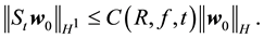
Condition 21. For any R and r with  there exist
 ,
,  ,
,  all positive and there exists an integer
  such that
 (19)
(19)
 (20)
(20)
where  for all k.
Condition 22. For any  there is a decreasing sequence
  as
as  such that
 (21)
(21)
where  is the projection onto the first N eigenfunctions
 .
.
Assume the kicked flow also satisfies:
Condition 23. For K, the support of the distribution of ,
,

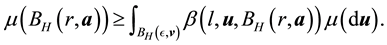
and for any B bounded in H let
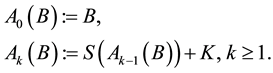 (22)
(22)
Then there exists  such that for any B there is
  such that:
 (23)
(23)
In addition, assume that the kicked flow satisfies the following type of controllability.
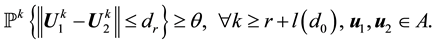
Condition 24. For any d > 0 and R > 0 there exists integer  and real number
  such that
 (24)
(24)
In other words, the kicked flow from two different initial conditions has a positive probability of becoming arbitrarily close together in finite time.
We now formulate a modified version of Theorem 3.2.5 from [12] .
Theorem 25. If the forced-kicked system (13) satisfies Conditions 21, 22, 23, and 24 and the kicks satisfy Condition 15 then there is  such that if
  for all
 , there exists an unique invariant measure, and for any
  there is
  such that for any real-valued Lipschitz function h on H

The constant  is a constant not dependent on h, u, R, or k. (
 is the standard Lipschitz norm.)
While Theorem 25 can be proved using the same approach as in [7] , we instead use an approach similar to that in [2] [6] [12] to highlight the dependence on the conditions. Though [12] uses external force f = 0 and [6] only allows a time-independent force and we are considering time-periodic forces here, there are only two main differences in the above conditions and the ones in [12] : the inequalities now depend on the norm of f and the use of Condition 24. Due to these slight differences, a brief sketch of the proof of Theorem 25 based on the arguments found in [2] [17] is given (summarized well in [7] , p. 10). The main idea behind the argument is the following lemma ([12] , Lemma 3.2.6 or [7] , Prop. 2.5).
Recall that a pair of random variables  defined on a probability space is called a coupling for the given measures
  if the distribution of
  is
is ,
, 
Lemma 3. Under the conditions of Theorem 25, there exists a constant  such that for any points
  with
with  the measures
  admit a coupling
  such that
where C > 0 does not depend on .
.
Since the conditions on the deterministic solution operator are imposed on each fixed time interval and the operator is the same for each interval, the kicked-equations have the same form as the time-independent and zero-force cases. Thus, with the exception that constants now depend on the norm of the deterministic force, the proof of Lemma 3, which depends on conditions 20 and 21, is identical to the proof in [12] .
It should be noted that the choice of N in Theorem 25 comes from the construction of the coupling in Lemma 3 and the construction only needs that N is sufficiently large.
Remark 26. In [7] the complication in proving Lemma 3 lies not in the choice of a time-periodic deterministic force, but the choice of random perturbation.
Given Lemma 3, the remainder of the proof proceeds under the following two cases:
1) If  for d small enough, by Lemma 3, there is a positive probability that the random variables after one time step are within
 . By iteration there is a positive probability that the random variables will be within
  after n time steps.
2) If  instead then, by Condition 24, there exists a finite time l where
 . After this, Lemma 3 again implies that the distance between the random variables is continually halved with positive probability.
The above argument gives the main idea behind the following lemma ([2] , Lemma 3.3):
Lemma 4. Let , where A is the invariant set, and
 . Then under the condition of Theorem
25 for any  the measures
  admit a coupling
  such that
1) The maps  are measurable with respect to
 .
.
2) There exists a constant  not depending on
  and k such that
 (25)
(25)
3) If  then
then
 (26)
(26)
Due to Lemma 3 which establishes the existence of a coupling, the proof of this lemma is very similar to the one in [2] . The main difference is the use of Condition 24 here instead of Lemma 3.1 in [2] which assumes that all solutions converge to 0 since the deterministic forcing is 0 there. The remainder of the proof of Theorem 25 follows identically to the argument in [17] .
Having established Theorem 25, it only remains to check that the conditions hold for the kicked Navier- Stokes equations. It is straightforward that Condition 21 implies Condition 23. Furthermore, since Conditions 21 and 22 are well known and analogous to results for the torus these are included in the Appendix for completion. Instead only Condition 24 is proved here.
3.3. Proof of Condition 24
In order to establish Condition 24 the following is needed ([1] , Lemma 5.4), which establishes that a sequence of realizations of kicks can be taken arbitrarily close to any prescribed sequence of vectors in  with positive probability.
Lemma 5. For any  and any integer
 , there is a
  such that
uniformly in  in
in  where
where  is the support of the distribution of the kicks.
The proof of Condition (24) uses the main idea behind Lemma 3.1 in [2] and is split into the two cases considered.
Lemma 6. Suppose that there exists an asymptotically stable solution, then for any d > 0 and R > 0 there exists integer  and real number
  such that

Proof. First fix all realization of the kicks as the zero realization. Then by assumption there exists a time l such that
 (27)
(27)
By continuity of the flow there is a  small enough that if
  for
for  then
then
 (28)
(28)
By Lemma 5 the probability of  is nonzero. Thus
 (29)
(29)
as desired.
Now recall that the N in Theorem 25 is from the construction of the coupling in Lemma 3. Let N' be the maximum of the N from the big kick assumption (and thus ³ M) and the N generated by Lemma 3.
Lemma 7. Let  for
for . Suppose that there exists a finitely stable point u and assume that the big kick assumption holds, then for any d > 0 and R > 0 there exists an integer
  and real number
  such that

Proof. Let δ be the radius for the finitely stable point, u, and fix all realizations of the kicks as the zero realization. By (53) there exists a time l such that
 (30)
(30)
By the big kick assumption, there exists a kick  such that
 (31)
(31)
Again fix all realizations as the zero realization. By the assumption of a finitely stable point, there exists a time k such that
 (32)
(32)
Thus there exists a time  such that
 (33)
(33)
By continuity,  can be chosen such that if
  for
for ,
,  where
where  is another realization of the kick, and
  for
for  then
then
 (34)
(34)
By Lemma 5 there is a positive probability of the kicks satisfying the inequalities.
This completes the proof of Condition 24 and thus there is uniqueness of invariant measure in H.
4. Support of the Measure
Before stating the main result of this section, we recall some definitions and straightforward results about the support of a measure.
Definition 27. The support of a measure  on H is the smallest closed subset K in H such that
  . A measure is concentrated on a set B if
 .
.
To continue we need Lemma 5.5 from [1] .
Definition 28. For , let
, let . Then the set of attainability from the set y at time n is defined as
 . The set of attainability from y is defined as
The set of attainability for a set of points is the union of the set of attainability for all points in the set.
Lemma 8. For any  there is an integer
  such that
  is contained in the r-neighborhood of
 , i.e. for any
  there exists
  such that
 , where
  is the ball of radius r in H centered at a.
It is worth noting that the definition of the set of attainability is similar to Condition 23 except that the ball is centered at y instead of 0.
Remark 29. The support of the measure for the Navier-Stokes equations is concentrated on V ([6] , Lemma 5.5.2) and, in general, the support of the measure is contained in a ball centered around the origin of radius the square root of
 (35)
(35)
where  for all k ([6] , Lemma 5.5.3).
When there is an asymptotically stable solution the support is contained in a ball of radius
 (36)
(36)
centered at the limiting solution ([6] , Lemma 5.2.1), where L is the rate of convergence, i.e.  for
for .
.
Support of the Measure
We next extend the standard definitions of wandering and nonwandering points ([18] , page 27) to the case of stochastic flow.
Definition 30. Let  A point
  is nonwandering if for all
  and for every
  there exists
  such that

Definition 31. A point  is wandering if there exists
  and there exists
  such that for all

A point is defined as wandering or nonwandering based on the behavior of nearby points. One consequence of this is that for a stationary force an unstable stationary solution is now a wandering point unlike for the deterministic setting.
The following result was proved in [6] , Theorem 5.5.8.
Theorem 32. Let A be the set of attainability from the the set of nonwandering points. Then any  is in the support of the measure.
We outline the proof below (which is similar to the steps in [1] , p. 320). Note that it is necessary to establish that  for any
 .
.
・ By time-invariance, for any , for any
  and any
 (37)
(37)
Thus, by integrating over a subset of H instead
 (38)
(38)
・ Thus, it is sufficient to show that for any  there exists
 ,
,  , and times t1, t2 such that
 (39)
(39)
・ By the definition of the set of attainability, there is a nonwandering point y such that a is accessible from y. Furthermore, since for any 
 (40)
(40)
it is enough that  and
and  are strictly positive, which follows from the next two lemmas.
Lemma 9. Let y be a nonwandering point. For any  there is
 , an integer
 , and a constant
  such that
The proof is very similar to that of Condition 24 and thus only a sketch is given. By the definition of a nonwandering point, the intersection of any open ball (for example of radius ) around a nonwandering point, y,
has a non-empty intersection with the deterministic flow of the set at some time , i.e. if
  then
then
 . By continuity, there exists
  such that if the initial condition
  and the kicks are small enough then
  (see [6] , Lemma 5.5.11 or [1] , p. 321-322).
Lemma 10. Let A be the set of attainability from the set of nonwandering points. For any  and any
  there exists
  and a nonwandering point y such that for some time t2 and all
 ,
,
The proof is nearly a repeat of the argument made in [1] , page 322, with modifications for the change in the definition of the set of attainability, so only a brief sketch is given. By Lemma 8, there is  such that
  is attainable by a finite sequence of fixed kicks from the nonwandering point y. By continuity of the flow and the properties of the kicks, there is a
  and
and  such that if
  and the kicks vary by at most
  then there is a positive probability that
 .
.
Due to the existence of an asymptotically stable solution when the force is small enough, gives a zonal solution, or gives an almost zonal solution, the following holds.
Corollary 1. If the force
1) is small enough―see Remark 33;
2) yields a zonal solution;
3) yields an almost zonal solution;
then the support of the measure is the set of attainability from the unique exponentially stable periodic solution.
5. Conclusions
While there is invariant measure for the kicked Navier-Stokes equations with a bounded time-periodic deterministic force, it is only possible to give a clear description of the support of the measure in a few limited situations. Furthermore, if there is an asymptotically stable solution then the support can be considered to nearly be the unique stable periodic solution since the kicks can be taken arbitrarily small (with the first N dimensions nonzero). Unfortunately, for more general forces the support of the measure is not as clear. For example, it is not as clear what nonwandering points may exist. In addition, while the assumption of a finitely stable point is more general than the assumption of a globally attracting solution and gives that there is a (at least one) periodic solution (possibly with the same period as the force), the size requirement on the kick is problematic both for understanding the support of the measure and for meteorological considerations.
It is possible, however, that the kicks may be allowed to be smaller. The big kick assumption is introduced to ensure that a kick can, with positive probability, send the flow into the neighborhood of any point in the deterministic absorbing ball. The necessity of the big kick assumption comes from the deterministic setting where a Dirac measure at any stationary solution is a time-invariant measure, giving non uniqueness if there are multiple stationary solutions. Thus, for example, if there are two stable stationary solutions the kicks must be (at minimum) large enough to send the flow from inside the radius of stability of one into the radius of stability of the other. The big kick assumption is sufficient to do this, but a smaller kick may suffice.
Of course, the results presented in this paper also apply to time-independent and zero forcing deterministic forces since they are trivially time-periodic. Furthermore, the majority of the results presented in this paper apply to the Navier-Stokes equations on the torus. For example, while a zonal and almost zonal solution no longer makes sense on the torus, if the force still yields an unique asymptotically stable solution then the support of the measure is again straightforward to describe.
Acknowledgements
We thank the Editor and the referee for their comments.
Cite this paper
GregoryVarner, (2015) Unique Measure for the Time-Periodic Navier-Stokes on the Sphere Navier-Stokes on the Sphere. Applied Mathematics,06,1809-1830. doi: 10.4236/am.2015.611160
References
- 1. Kuksin, S. and Shirikyan, A. (2000) Stochastic Dissipative PDE’s and Gibbs Measures. Communications in Mathematical Physics, 213, 291-330.
http://dx.doi.org/10.1007/s002200000237 - 2. Kuksin, S. and Shirikyan, A. (2001) A Coupling Approach to Randomly Forced Nonlinear PDE’s. I. Communications in Mathematical Physics, 221, 351-366.
http://dx.doi.org/10.1007/s002200100479 - 3. Kuksin, S. and Shirikyan, A. (2006) Randomly Forced Nonlinear PDEs and Statistical Hydrodynamics in 2 Space Dimensions. European Mathematical Society, Zürich.
http://dx.doi.org/10.4171/021 - 4. Kuksin, S. and Shirikyan, A. (2002) Coupling Approach to White-Forced Nonlinear PDEs. Journal de Mathématiques Pures et Appliquées, 81, 567-602.
http://dx.doi.org/10.1016/S0021-7824(02)01259-X - 5. Shirikyan, A. (2005) Ergodicity for a Class of Markov Processes and Applications to Randomly Forced PDE’s. I. Russian Journal of Mathematical Physics, 12, 81-96.
- 6. Varner, G. (2013) Stochastically Perturbed Navier-Stokes System on the Rotating Sphere. PhD Dissertation, The University of Missouri, Columbia.
- 7. Shirikyan, A. (2015) Control and Mixing for 2D Navier-Stokes Equations with Space-Time Localised Noise. Annales Scientifiques de l’ENS, 48, 253-280.
- 8. Brzezniak, Z., Goldys, B. and Le Gia, Q.T. (2015) Random Dynamical Systems Generated by Stochastic Navier-Stokes Equation on the Rotating Sphere. Journal of Mathematical Analysis and Applications, 426, 505-545.
http://dx.doi.org/10.1016/j.jmaa.2015.01.054 - 9. Il’in, A.A. (1991) The Navier-Stokes and Euler Equations on Two-Dimensional Closed Manifolds. Mathematics of the USSR-Sbornik, 69, 559-579.
http://dx.doi.org/10.1070/SM1991v069n02ABEH002116 - 10. Ilyin, A. (2004) Stability and Instability of Generalized Kolmogorov Flows on the Two-Dimensional Sphere. Advances in Differential Equations, 9, 979-1008.
- 11. Dymnikov, V. and Filatov, A. (1997) Mathematics of Climate Modeling. Birkhäuser, Boston.
- 12. Kuksin, S. and Shirikyan, A. (2012) Mathematics of Two-Dimensional Turbulence. Cambridge University Press, New York.
http://dx.doi.org/10.1017/CBO9781139137119 - 13. Robinson, J. (2001) Infinite-Dimensional Dynamical Systems. Cambridge University Press, New York.
http://dx.doi.org/10.1007/978-94-010-0732-0 - 14. Heywood, J. and Rannacher, R. (1986) An Analysis of Stability Concepts for the Navier-Stokes Equations. Journal für die Reine und Angewandte Mathematik, 372, 1-33.
- 15. Furshikov, A. and Vishik, M. (1988) Mathematical Problems of Statistical Hydromechanics. Kluwer Academic Publishers, Boston.
- 16. Lions, J.L. and Magenes, E. (1972) Non-Homogeneous Boundary Value Problems, II. Spring-Verlag, Heidelberg and New York.
- 17. Kuksin, S., Piatnitski, A. and Shirikyan, A. (2002) A Coupling Approach to Randomly Forced Nonlinear PDE’s. II. Communications in Mathematical Physics, 230, 81-85.
http://dx.doi.org/10.1007/s00220-002-0707-2 - 18. Dymnikov, V. and Filatov, A. (1997) Mathematics of Climate Modeling. Birkh?user, Boston.�
- 19. Il’in, A.A. (1994) Partly Dissipative Semi-Groups Generated by the Navier-Stokes System on Two-Dimensional Manifolds, and Their Attractors. Russian Academy of Sciences. Sbornik Mathematics, 78, 159-182.
http://dx.doi.org/10.1070/sm1994v078n01abeh003458 - 20. Skiba, Y. (2012) On the Existence and Uniqueness of Solution to Problems of Fluid Dynamics on a Sphere. Journal of Mathematical Analysis and Applications, 388, 627-644.
http://dx.doi.org/10.1016/j.jmaa.2011.10.045
Appendix
A.1. Estimates
We now present estimates that will be needed to establish Conditions 21 and 22 and Lemmas 1 and 2. With the exception of Equations (48) and (49) of Lemma 12 and Lemma 13 these estimates are analogous to standard estimates on flat-domains with periodic boundary conditions.
Lemma 11. For  the Poincare Inequality holds, i.e.
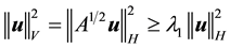 (41)
(41)
where  is the first eigenvalue of the Laplacian. In particular, the V-norm is equivalent to the H1-norm on V.
The proof is identical to the case of flat domains due to the existence of an orthonormal basis. Furthermore,  is the first eigenvalue of the scalar Laplacian on the sphere ([9] , p. 567).
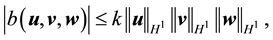
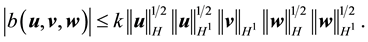
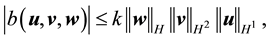
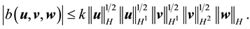
Lemma 12. For , the trilinear form satisfies
 (42)
(42)
 (43)
(43)
 (44)
(44)
If  then
then
 (45)
(45)
 (46)
(46)
 (47)
(47)
Furthermore, let 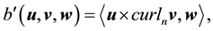 be a zonal vector field (only latitudinal dependence) and
  then
then
 (48)
(48)
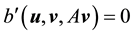 (49)
(49)
Proof. Since the proof of (42) and (45) are identical to the ones in [9] , pp. 566-568, the proofs of (43), (44), (46), and (47) follow from applying the Hölder inequality and the Ladyzhenskya inequality after taking extensions ([9] , pp. 566-567) and the proof of (48) is identical to the calculation on p. 69 of [19] (which uses Lemma 4.4 on p. 62 there), we will only prove (49) here.
Since the sphere is simply connected, for a divergence-free vector field u, there is a flow function 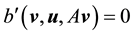 ([9] , pp. 567-568)

where ∆ is the spherical Laplacian for functions.
For the following calculation, we will need the following information about the spherical Jacobian ([19] p. 51)

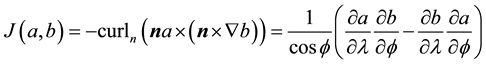 by Stoke’s Theorem. (50)
The proof of Equation (49) uses an argument similar to [19] , p. 70. Recall that  and denote the flow functions for u and v as
  and
and , respectively.
 (51)
(51)
The following lemma will allow for the Coriolis term  to vanish from all the estimates. Its proof only uses that the Laplacian commutes with differentiability in the longitudinal direction―see [20] , p. 635.
Lemma 13. For smooth vector fields u, the following holds for 
 (52)
(52)
We now turn to the proofs of Conditions 21 and 22 and Lemmas 1 and 2. Since many of the calculations are standard, only the main steps are given. Recall that .
.
A.2. Proof of Condition 21
Let  be the solution of the 2D Navier-Stokes equations with initial condition
  at time t.
Lemma 14. The following inequalities hold for the deterministic 2D Navier-Stokes equation on the sphere for all :
:
 (53)
(53)
 (54)
(54)
where  is the first eigenvalue of the operator −∆ on functions.
Moreover, for any 
 (55)
(55)
Proof. The proof follows the estimates in [9] , p. 572. Take the L2 inner product of the Navier-Stokes equation with u. By (52) and (42)
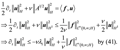 (56)
(56)
This gives
 (57)
(57)
establishing (53).
For (54), take the L2 inner product with Au. By (52) and (45)
 (58)
(58)
Therefore
 (59)
(59)
establishing (54).
For (55), note that integrating (56) from  to
to  gives
gives
 (60)
(60)
(54) implies that for any  and any
 (61)
(61)
Integrating (61) with respect to  from
from  to t gives, using (60) and (53)
 (62)
(62)
establishing (55).
Now consider the difference between two solutions 
 (63)
(63)
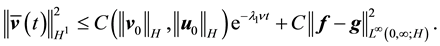
Lemma 15. For any  and for all
  the difference of solutions satisfies
 (64)
(64)
whenever  and
and .
.
Proof. Taking the L2 inner product with w
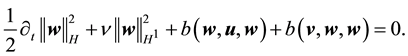 (65)
(65)
By (42) and (44),
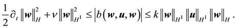 (66)
(66)
By the Cauchy inequality
 (67)
(67)
and thus by (41)
 (68)
(68)
By (60)
 (69)
(69)
Thus the exponential is less than or equal to some constant (depending on R and the norms of f) for any fixed .
.
Remark 33. By (69) in order to ensure (16) it is sufficient that

If Equation (16) is satisfied, there is a unique globally exponentially stable solution that is periodic with the same period as the force.
A.3. Proof of Condition 22
Lemma 16. Let  and for any
  let
let  and
and . The following estimate holds for all
 :
:
 (70)
(70)
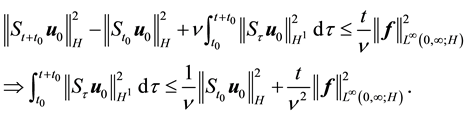
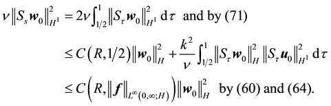
Proof. Integrating (58) from s to t gives
 (71)
(71)
Using (55) gives for 
 (72)
(72)
Integrating (67) from 1/2 to 1 and by the Mean Value Theorem there is  such that
 (73)
(73)
Taking the L2 inner product of (63) with Aw gives
 (74)
(74)
By (47) and (46) respectively, the right side of (74) is bounded above by
 (75)
(75)
Therefore
 (76)
(76)
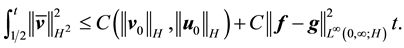
and
 (77)
(77)
By (53) and (72) this is bounded above by
 (78)
(78)
By (60) and (73) this is bounded above by
 (79)
(79)
which establishes (70).
Let .
.
Then
 (80)
(80)
where the last step is by (70). For any t ≥ 1 a N can be found (depending on t, R, and f) such that the  is less than or equal to any q > 0. Since t = 1 for the kicked equations, N can be chosen only depending on R and f.
A.4. Proof of Lemma 1
The proof is analogous to a calculation in [19] , pp. 69-70 (done for ), and the steps given in [6] , Lemma 5.3.2, where a general time-independent zonal force is considered.
Let  solve the time-dependent Navier-Stokes equations with forcing f where u' is a perturbation and
  is the zonal solution. The perturbation solves
 (81)
(81)
where
 (82)
(82)
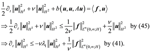
Dropping the primes for ease of notation and taking the inner product with Au gives
 (83)
(83)
 by (52), (48), and (49). Thus for any
  the perturbation satisfies
 (84)
(84)
Since , (55) gives
 (85)
(85)
Thus the solution is asymptotically attracting in H.
A.5. Proof of Lemma 2
The proof uses a different approach than the analogous result in [6] , Proposition 5.4.1 which gives a much more direct argument here. Instead we show that if the solution to the Navier-Stokes equations with a nonzonal force is “close enough” to the zonal solution, then it is globally exponentially stable. We then use standard estimates to the express the inequalities in terms of the distance from the force f.
Let u be the unique zonal solution for the Navier-Stokes equations with force f. Suppose g is such that there exists 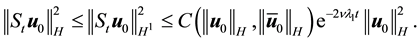 that solves
 (86)
(86)
Let 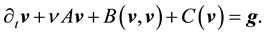 be another solution to (86) and consider
  which solves
 (87)
(87)
Rewriting the nonlinear terms gives
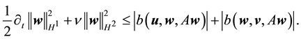
 (88)
(88)
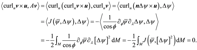
Take the inner product with Aq. By (45) 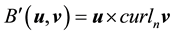 and since u is zonal
  and
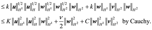
and  by (48) and (49). By Equations (46), (47), and the Cauchy inequality the trilinear terms
 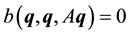 and
and  satisfy

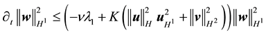
Thus
 (89)
(89)
For any 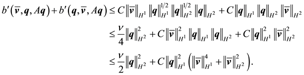 integrating (89) on
 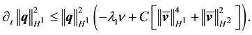 gives
gives
 (90)
(90)
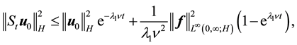
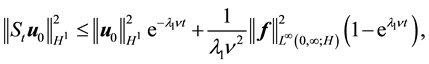
Since  by (55)

Thus if the norms of  are small enough then the unique solution v is globally exponentially stable in H1 (and thus in H).
It remains to express the norms of 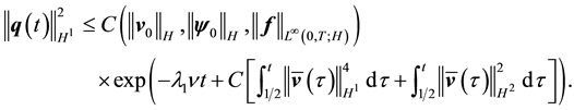 in terms of the difference of forces. Since
 , consider the difference between the Navier-Stokes equations with force f and zonal solution u and Equation (86) getting
 (91)
(91)
Since  and since u is zonal, the inner product with
  and Equations (45), (48), and (49) give
 (92)
(92)
Integrating from , using
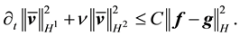 , and (55) gives
 (93)
(93)
Similarly using (41) and integrating (92) from 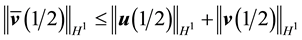 yields
 (94)
(94)
Thus by Cauchy’s inequality
 (95)
(95)
Thus the term in the exponential in (90) is bounded above by
Therefore there is 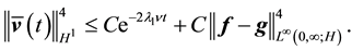 such that if
  then the unique solution v is globally exponentially stable in H.