Advances in Applied Mathematics
Vol.
08
No.
10
(
2019
), Article ID:
32785
,
16
pages
10.12677/AAM.2019.810196
A Literature Review and Application of Sev Eral Generalized Function Expansion Methods in Constructing Exact Solutions of Partial Differential Equations -Expansion Method, -Expansion Method Construction (2 + 1) Exact Solution of the Dimensional Boiti-Leon-Pempinelli Equation
Dashan Wu, Yuhuai Sun, Lingxi Du
College of Mathematics Science, Sichuan Normal University, Chengdu Sichuan

Received: Oct. 8th, 2019; accepted: Oct. 24th, 2019; published: Oct. 31st, 2019

ABSTRACT
First, the system gives -expansion method, F-expansion method, -expansion method, improved Kudryashov method, direct truncation method, to construct the literature review of the origin and research status of the exact solutions of partial differential equations. Next, the steps of constructing the exact solutions of the partial differential equations by the above five generalized function expansion methods are given in comparison. Finally, through the above five generalized -expansion method, -expansion method in the function expansion method constructs the exact solution of the (2 + 1)-dimensional Boiti-Leon-Pempinelli equation. The control variable method is used to analyze the influence of three variables on the exact solution in the (2 + 1)-dimensional Boiti-Leon-Pempinelli equation.
Keywords: -Expansion Method, F-Expansion Method, -Expansion Method, Improved Kudryashov Method, Direct Truncation Method, (2 + 1) Dimension Boiti-Leon-Pempinelli Equation, Exact Solution, Mathematical Experiment

几种广义的函数展开法在构建偏微分方程 精确解中的文献综述与应用 -展开法、 -展开法构建(2 + 1)维Boiti-Leon-Pempinelli方程精确解
吴大山,孙峪怀,杜玲禧
四川师范大学,数学科学学院,四川 成都

收稿日期:2019年10月8日;录用日期:2019年10月24日;发布日期:2019年10月31日

摘 要
首先,系统给出 -展开法、F-展开法、 -展开法、改进的Kudryashov方法、直接截断法,构建偏微分方程的精确解的起源与研究现状的文献综述。接下来,采用对比方式给出上述五种广义的函数展开法在构建偏微分方程精确解的步骤。最后,通过上述五种广义的函数展开法中的 -展开法、 -展开法构建(2 + 1)维Boiti-Leon-Pempinelli方程的精确解,并使用控制变量法进行数学实验分析了(2 + 1)维Boiti-Leon-Pempinelli方程中三个变量对于精确解的影响。
关键词 : -展开法,F-展开法, -展开法,改进的Kudryashov方法,直接截断法, (2 + 1)维Boiti-Leon-Pempinelli方程,精确解,数学实验

Copyright © 2019 by author(s) and Hans Publishers Inc.
This work is licensed under the Creative Commons Attribution International License (CC BY).
http://creativecommons.org/licenses/by/4.0/


1. 引言
偏微分方程精确解可以很好的描述物理、工程等方面的各种模型,因此,偏微分方程精确解的构建问题一直都是热点问题,偏微分方程精确解的构建目前有很多方法。如,Bäcklund变换 [1] [2] [3] [4] [5],Darboux变换 [6] [7] [8] [9] [10],齐次平衡法 [11] [12] [13] [14] [15],首次积分法 [16] [17] [18] [19] 以及各种广义的函数展开法。使用函数展开法构建偏微分方程精确解有几十种,本文以(2 + 1)维Boitl-Leon-Pempinelli
方程为例,比较分析 -展开法、F-展开法、 -展开法、Kudryashov方法、直接截断法在构建偏微分方程精确解的异同。下面给出上述五种广义的函数展开法,构建偏微分方程的精确解的起源与研究现状的文献综述。
-展开法,是Li Wen-An等借助Chun Quanbian在文献 [20] 提出的基础之上,在文献 [21] 提出的 -展开法而形成的,并用 -展开法构建出了Vakhncnko方程的精确解,其后在文献 [22] - [28] 中, -展开法被运用在求解各种方程的精确解中。
F-展开法,2003年由Y.B. Zhou等在文献 [29] 中首次提出并构建出了一个耦合Kdv方程的精确解,之后王明亮,斯仁道尔吉在文献 [30] [31] [32] 使用F-展开法KdV方程的精确解与广义Nizhnik-Novikov-Veselov方程组的精确解。
-展开法,是由Ji-Huan He和Xu-Hong Wu在文献 [33] 首次提出,在文献 [34] [35] [36] [37],分别使用 -展开法构建出了Konno-Oono方程,(2 + 1)-维Sawada-Kotera(SK)方程与(3 + 1)-维非线性evolution方程的精确解。
Kudryashov方法,由Kudryashov NA于1988年在文献 [38] 中提出,之后Anonymous在文献中将其运用到构建偏微分方程的精确解中,之后文献 [39] [40] [41] 分别使用改进的Kudryashov方法构建出了high-order nonlinear Schrödinger方程,nonlinear transmission line方程与Fractional nonlinear evolution方程的一系列精确解。
直接截断法,由赵等人在文献 [42] [43] 提出,之后文献 [44] 提出了离散区间系统降阶的直接截断方法,董长紫,刘转玲等在文献 [45] [46] [47] 使用直接截断法构建出了Klein-Gordon方程,高次非线性薛定谔方程与Burgers方程的精确解。
对于如下(2 + 1)维Boiti-Leon-Pempinelli方程(1):
(1)
在文献 [48] 通过Khater方法构建出了方程(1)大量三角函数解、双曲函数解,在文献 [49] 通过动力系统和数值模拟其不同拓扑结构的相图,通过计算复杂的椭圆积分,获得了方程(1)椭圆函数类型的周期波解,在文献 [50] 使用扩展映射方法构建出了方程(1)的精确解,在文献 [51] 使用 -展开法构建出了方程(1)的有理函数解、双曲函数解、三角函数解。在文献 [52] 使用Bäcklund变换,在文献 [53] 使用广义Riccati方程方法,在文献 [54] 使用扩展的tanh方法,在文献 [55] 使用了进一步扩展tanh的方法,获得了方程(1)的各类精确解。在文献 [56] [57] 分别使用改进的伯努利子方程函数法与对称约化法构建了方程(1)的大量精确解。
在接下来将具体描述 -展开法、F-展开法、 -展开法、改进的Kudryashov方法、直接截断法、构建(2 + 1)维偏微分方程精确解的过程结果,同时使用 -展开法、 -展开法构建(2 + 1)维Boiti-Leon-Pempinelli方程的精确解,并使用控制变量法进行数学实验分析了(2 + 1)维Boiti-Leon-Pempinelli方程中三个变量对于精确解的影响。
2. 方法描述
考虑含有三个个独立变量 的时空分数阶偏微分方程如下:
(2)
其中p是关于 及其偏导数的多项式。对上述方程(2)作如下的行波变换:
(3)
将(2)转化为常微分方程:
(4)
其中 , 为u关于 的一阶导数,二阶导数。
2.1. -展开法构建偏微分方程精确解描述
步骤1:假设(4)有如下形式的解:
(5)
其中 满足:
(6)
其中 为待定常数, 通过齐次平衡法确定。
步骤2:将(6)代入(5),合并 的同类项,并令各项系数为零求解关于 的代数方程组, 为待定常数, 。
步骤3:结合(5)解关于代数方程组满足:
(7)
其中 是常数。
步骤4:将 和 代入(7)得到(1)的精确解。
2.2. F-展开法构建偏微分方程精确解描述
步骤1:假设(4)有如下形式的解:
(8)
其中 为常数, 。 满足:
(9)
同时系数 和 在 时满足表1 (参见文献 [29] )。
步骤二:将(8)代入(4)通过齐次平衡法确定n,借助(9)与表1得到关于 的代数多项式,令 的各次项系数为零,得到关于 的代数方程组。
步骤三:解步骤三获得的代数方程组,使用 解出 ,代入(8)就得到方程(1)的行波解。
2.3. (exp)-展开法构建偏微分方程精确解描述
步骤一:假设方程(4)有如下形式的解:
(10)
其中, 是待定常数, 。 通过齐次平衡法确定。 满足:
(11)
方程(11)有以下形式解:
(12)
步骤二:将(11)代入(10)合并 相同项的系数,并令相同项系数为零,得到关于 的代数方程组,并结合(12)可得方程(1)的精确解。
2.4. 改进的Kudryashov方法构建偏微分方程精确解描述
步骤一:假设方程(4)有如下形式的解:
(13)
其中, 是待定常数, 。 通过齐次平衡法确定。
(14)
满足:
(15)
方程(15)有以下解:
(16)
由(13),(15)可得:
(17)
步骤二:将(16),(14)和(13)代入(4)合并 ,相同项的系数,并令相同项系数为零,得到关于 的代数方程组,并结合(12)可得方程(1)的精确解。
2.5. 直接截断法构建偏微分方程精确解描述
步骤一:假设方程(4)有如下形式的解:
(18)
并且 形式为:
(19)
其中 为待定参数, 借助方程(4)由齐次平衡法确定。
满足以下椭圆函数条件:
(20)
步骤二:将(17),(18)与(19)代入(4)可得关于 的多项式,令 的系数和常数项为零,得到一个代数方程组,求解关于参数 的方程组。
步骤三:根据(17),(18)得到方程(1)的精确解。
3. 应用两种广义的函数展开法构建构建(2 + 1)维Boiti-Leon-Pempinelli方程精确解
下面以上述五种方法中的 -展开法与 -展开法为例,构建(2 + 1)维Boiti-Leon-Pempinelli方程(1)的精确解。首先将方程(1)进行如下的行波变换:
(21)
对方程(1)的第一个方程积分一次并取积分常数为零,代入方程(1)第二式得到常微分方程:
(22)
其中 为常数。平衡最非线性项 和最高阶导数项 ,则有: ,有 。
3.1. -展开法构建(2 + 1)维Boiti-Leon-Pempinelli方程精确解
由 则式(22)有如下形式的解
(23)
其中 满足式(6),将(23)代入(22),由(23)结合(6)可得:
(24)
将 和 代入方程(22)中,并平衡 ,并令各幂次的系数为零,得到关于 的代数方程组:
(25)
解上述代数方程组,并结合方程(7),方程(23)作如下讨论:
情况一:
(26)
当 ,得到三角函数解:
(27)
当 ,得到双曲函数解:
(28)
当 ,得到有理函数解:
(29)
情况二:
(30)
当 ,得到三角函数解:
(31)
当 ,得到双曲函数解:
(32)
当 ,得到有理函数解:
(33)
其中 , 为积分常数, 为实数, 。
3.2. (exp)-展开法构建(2 + 1)维Boiti-Leon-Pempinelli方程精确解
下面应用 -展开法来构建(2 + 1)维Boiti-Leon-Pempinelli方程(1)精确解。由 结合(10)式知方程(1)如下形式的解
(34)
由方程(10),(34),可得:
(35)
将 和 代入方程(22)中,并合并 相同项的系数,并令相同项系数为零,得到关于 的代数方程组:
(36)
解上述代数方程组,并结合方程(12),方程(34)作如下讨论:
情况一:
(37)
当
(40)
当
(41)
当
(42)
当
(43)
当
(44)
情况二:
(45)
当
(46)
当
(47)
当
(48)
当
(49)
当
(50)
其中 ,c为积分常数, 实数, 。
4. 数学实验与精确解的图形
下面使用控制变量法,以解 为例,做出 取 在x-y-t坐标系下的3D图形如图(1)。

Figure 1. the x-y-t of 3D figures
图1. 在x-y-t的3D图形
取 在x-o-t坐标系下(取 )的图形如图(2),在x-o-y坐标系下(取 )的图形如图(3)。
取 在y-o-t坐标系下(取 )的图形如图(4),在x-y坐标系下(取 )的图形如图(5)。
取 在x-t坐标系下(取 )的图形如图(6),在y-t坐标系下(取 )的图形如图(7)。

Figure 2. the x-o-t (t = 1) of 3D figures
图2. 在x-o-t (t = 1)的3D图形

Figure 3. the x-o-y (t = 1) of 3D figures
图3. 在x-o-y (t = 1)的3D图形
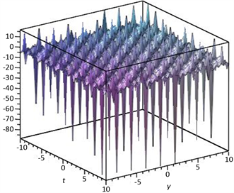
Figure 4. the y-o-t (t = 1) of 3D figures
图4. 在y-o-t (t = 1)的3D图形

Figure 5. the x-y (t = 1) of figures
图5. 在x-y (t = 1)的3D图形

Figure 6. the x-t (t = 1) of figures
图6. 在x-t (t = 1)的图形

Figure 7. the x-t (t = 1) of figures
图7. 在x-t (t = 1)的图形
实验结论:通过上述实验比较图(2)与图(4),图(6)与图(7)发现(2 + 1)维Boiti-Leon-Pempinelli方程(1)中三个变量 对于精确解结构的影响一致,这也就是(1 + 1)维Boiti-Leon-Pempinelli方程被广泛研究的原因。比较图(3)与图(2)、图(4)或者比较图(5)与图(6)、图(7)知道(2 + 1)维Boiti-Leon-Pempinelli方程(1)变量t与变量 对于精确解结构的影响不一致。因此,就可以在下一步的工作中对(2 + 1)维Boiti-Leon-Pempinelli方程进行降低维数或者增加维数进行研究。
5. 结论
本文,给出 -展开法、F-展开法、 -展开法、改进的Kudryashov方法、直接截断法,构建偏微分方程的精确解文献综述共有57篇文献,同时给出了上述五种方法构建偏微分方程精确解的过程与结果,另外使用 -展开法构建出了(2 + 1)维Boiti-Leon-Pempinelli方程的精确解 ,这些解包括三角函数解,双曲函数解,有理函数解。使用 -展开法构建出了(2 + 1)维Boiti-Leon-Pempinelli方程的精确解 ,极大地丰富了(2 + 1)维Boiti-Leon-Pempinelli方程的精确解。
通过数学实验得到(2 + 1)维Boiti-Leon-Pempinelli方程中三个变量 对于精确解结构的影响一致,而变量t与变量 对于精确解结构的影响不一致。下一步的工作将继续使用这些广义的函数展开法构建分数阶偏微分方程或者随机偏微分方程的精确解。
基金项目
National Natural Science Foundation of China (国家自然科学基金,11371267);Natural Science Foundation of Sichuan Province of China (四川省自然科学基金,2012ZA135)。
文章引用
吴大山,孙峪怀,杜玲禧. 几种广义的函数展开法在构建偏微分方程精确解中的文献综述与应用(G′/G2)-展开法、(exp)-展开法构建(2 + 1)维Boiti-Leon-Pempinelli方程精确解
A Literature Review and Application of Sev Eral Generalized Function Expansion Methods in Constructing Exact Solutions of Partial Differential Equations(G′/G2)-Expansion Method,(exp)-Expansion Method Construction (2 + 1) Exact Solution of the Dimensional Boiti-Leon-Pempinelli Equation[J]. 应用数学进展, 2019, 08(10): 1659-1674. https://doi.org/10.12677/AAM.2019.810196
参考文献
- 1. Dodd, R.K. and Bullough, R.K. (1976) Bäcklund Transformations for the Sine-Gordon Equations. Proceedings of the Royal Society of London. Series A, Mathematical and Physical Sciences, 351, 499-523.
https://doi.org/10.1098/rspa.1976.0154 - 2. Fan, E.G. and Zhang, H.Q. (1980) A New Approach to Bäcklund Transformations of Nonlinear Evolution Equations. Applied Mathematics and Mechanics, 19, 645-650.
https://doi.org/10.1007/BF02452372 - 3. Fan, E.G. and Zhang, H.Q. (1980) Backlund Transformation and Exact Solutions for Whitham-Broer-Kaup Equations in Shallow Water. Applied Mathematics and Mechanics, 19, 713-716.
https://doi.org/10.1007/BF02457745 - 4. El-Shiekh, R.M. (2018) Painlevé Test, Bäcklund Transformation and Consistent Riccati Expansion Solvability for Two Generalised Cylindrical Korteweg-de Vries Equations with Variable Coefficients. Zeitschrift für Naturforschung A, 73, 207-213.
- 5. Gomes, J.F., Retore, A.L., Spano, N.I. and Zimerman, A.H. (2015) Backlund Transformation for Integrable Hierarchies: Example-mKdV Hierarchy. Journal of Physics: Conference Series, 597, Article ID: 012039.
https://doi.org/10.1088/1742-6596/597/1/012039 - 6. Matveev, V.B. (1979) Darboux Transformation and the Explicit Solutions of Differential-Difference and Difference-Difference Evolution Equations I. Letters in Mathematical Physics, 3, 217-222.
https://doi.org/10.1007/BF00405296 - 7. Zhou, Z.X. (1988) On the Darboux Transformation for (1+2)-Dimensional Equations. Letters in Mathematical Physics, 16, 83-92.
https://doi.org/10.1007/BF00398166 - 8. Huang, Y. (2013) Explicit Multi-Soliton Solutions for the KdV Equation by Darboux Transformation. IAENG International Journal of Applied Mathematics, 43, 135-137.
- 9. Qiu, D.Q. and Cheng, W.G. (2019) The N-Fold Darboux Transformation for the Kundu-Eckhaus Equation and Dynamics of the Smooth Position Solutions. Communications in Nonlinear Science and Numerical Simulation, 78, Article ID: 104887.
https://doi.org/10.1016/j.cnsns.2019.104887 - 10. Shi, D.D. and Zhang, Y.F. (2020) Diversity of Exact Solutions to the Conformable Space-Time Fractional MEW Equation. Applied Mathematics Letters, 99, Article ID: 105994.
https://doi.org/10.1016/j.aml.2019.07.025 - 11. 范恩贵, 张鸿庆. 非线性孤子方程的齐次平衡法[J]. 物理学报, 1998, 47(3): 353-362.
- 12. 范恩贵. 齐次平衡法、Weiss-Tabor-Carnevale法及Clarkson-Kruskal约化法之间的联系[J]. 物理学报, 2000, 49(8): 1409-1412.
- 13. Fan, E.G. (2000) Two New Applications of the Homogeneous Balance Method. Physics Letters A, 265, 353-357.
https://doi.org/10.1016/S0375-9601(00)00010-4 - 14. Wei, Y., He, X.-D. and Yang, X.-F. (2016) The Homogeneous Balance of Undetermined Coefficients Method and Its Application. Open Mathematics, 14, 816-826.
https://doi.org/10.1515/math-2016-0078 - 15. Stanbury, D.M. and Dean, H. (2019) Systematic Application of the Principle of Detailed Balancing to Complex Homogeneous Chemical Reaction Mechanisms. The Journal of Physical Chemistry A, 123, 5436-5445.
https://doi.org/10.1021/acs.jpca.9b03771 - 16. Fan, E.G. and Zhang, J. (2002) Applications of the Jacobi Elliptic Function Method to Special-Type Nonlinear Equations. Physics Letters A, 305, 383-392.
https://doi.org/10.1016/S0375-9601(02)01516-5 - 17. Feng, Z.S. (2002) On Explicit Exact Solutions to the Compound Burgers-KdV Equation. Physics Letters A, 293, 57-66.
https://doi.org/10.1016/S0375-9601(01)00825-8 - 18. 李林芳, 舒级, 文慧霞. 一类空时分数阶混合(1+1)维KdV方程的精确解[J]. 四川大学学报(自然科学版), 2018, 55(5): 912-916.
- 19. Arshed, S. and Arshad, L. (2019) Optical Soliton Solutions for Nonlinear Schrödinger Equation. Optik, 195, Article ID: 163077.
https://doi.org/10.1016/j.ijleo.2019.163077 - 20. Li, W.A., Chen, H. and Zhang, G.C. (2009) The -Expansion Method and Its Application to Vakhnenko Equation. Chinese Physics B, 18, 400-404.
https://doi.org/10.1088/1674-1056/18/2/004 - 21. Bian, C.Q., Pang, J., Jin, L.H. and Ying, X.M. (2010) Solving Two Fifth Order Strong Nonlinear Evolution Equations by Using the -Expansion Method. Communications in Nonlinear Science and Numerical Simulation, 15, 2337-2343.
- 22. 冯庆江, 杨娟. 应用改进的-展开法求广义变系数Burgers方程的精确解[J]. 山西师范大学学报(自然科学版), 2016, 30(2): 7-11.
- 23. 冯庆江, 雷学红. 应用-展开法求非线性发展方程的精确解(英文)[J]. 应用数学, 2013, 26(3): 538-543.
- 24. 石兰芳, 聂子文. 应用全新-展开方法求解广义非线性Schrödinger方程和耦合非线性Schrödinger方程组[J]. 应用数学和力学, 2017, 38(5): 539-552.
- 25. 冯庆江, 肖绍菊. 应用改进的-展开法求Zakharov方程的精确解[J]. 量子电子学报, 2015, 32(1): 40-45.
- 26. 孙鹏, 崔泽建. 展开法及其在KPP方程中的应用[J]. 西华师范大学学报(自然科学版), 2015, 36(4): 336-338+381.
- 27. 何姝琦, 陈立. 利用展开法求解KdV-Burgers方程和KdV-Burgers-Kuramoto方程[J]. 纺织高校基础科学学报, 2016, 29(3): 327-332.
- 28. 王思源, 陈浩. 求解KdV方程和mKdV方程的新方法: 展开法[J]. 华南师范大学学报(自然科学版), 2014, 46(1): 42-45.
- 29. Zhou, Y.B., Wand, M.L. and Wand, Y.M. (2003) Periodic Wave Solutions to a Coupled KdV Equations with Variable Coefficients. Physics Letters A, 308, 31-36.
https://doi.org/10.1016/S0375-9601(02)01775-9 - 30. 张金良, 王明亮, 王跃明. 推广的F-展开法及变系数KdV和mKdV的精确解[J]. 数学物理学报, 2006(3): 353-360.
- 31. 斯仁道尔吉. 通用F-展开法与nmKdV方程的精确解[J]. 内蒙古大学学报(自然科学版), 2018, 49(6): 561-566.
- 32. 扎其劳, 斯仁道尔吉. 利用F-展开法解广义Nizhnik-Novikov-Veselov方程组(英文)[J]. 内蒙古大学学报(自然科学版), 2005(6): 14-19.
- 33. He, J.-H. and Wu, X.-H. (2006) Exp-Function Method for Nonlinear Wave Equations. Chaos, Solitons and Fractals, 30, 700-708.
https://doi.org/10.1016/j.chaos.2006.03.020 - 34. Boz, A. and Bekir, A. (2008) Application of Exp-Function Method for (3 + 1)-Dimensional Nonlinear Evolution Equations. Computers and Mathematics with Applications, 56, 1451-1456.
- 35. Zayed, E.M.E., Amer, Y.A. and Al-Nowehy, A.-G. (2016) The Modified Simple Equation Method and the Multiple Exp-Function Method for Solving Nonlinear Fractional Sharma-Tasso-Olver Equation. Acta Mathematicae Applicatae Sinica, 32, 793-812.
https://doi.org/10.1007/s10255-016-0590-9 - 36. Shakeel, M., Mohyud-Din, S.T. and Iqbal, M.A. (2018) Modified Extended Exp-Function Method for a System of Nonlinear Partial Differential Equations Defined by Seismic Sea Waves. Pramana, 91, 28.
https://doi.org/10.1007/s12043-018-1601-6 - 37. Öziş, T. and Köroğlu, C. (2008) A Novel Approach for Solving the Fisher Equation Using Exp-Function Method. Physics Letters A, 372, 3836-3840.
https://doi.org/10.1016/j.physleta.2008.02.074 - 38. Kudryashov, N.A. (1988) Exact Soliton Solutions of the Generalized Evolution Equation of Wave Dynamics. Journal of Applied Mathematics and Mechanics, 52, 360-365.
https://doi.org/10.1016/0021-8928(88)90090-1 - 39. Taghizadeh, N., Mirzazadeh, M. and Mahmoodirad, A. (2013) Application of Kudryashov Method for High-Order Nonlinear Schrdinger Equation. Indian Journal of Physics, 87, 781-785.
https://doi.org/10.1007/s12648-013-0296-2 - 40. Hubert, M.B., Betchewe, G., Doka, S.Y. and Crepin, K.T. (2014) Soliton Wave Solutions for the Nonlinear Transmission Line Using the Kudryashov Method and the -Expansion Method. Applied Mathematics and Computation, 239, 299-309.
https://doi.org/10.1016/j.amc.2014.04.065 - 41. Ferdous, F. and Hafez, M.G. (2018) Oblique Closed form Solutions of Some Important Fractional Evolution Equations via the Modified Kudryashov Method Arising in Physical Problems. Journal of Ocean Engineering and Science, 3, 244-252.
https://doi.org/10.1016/j.joes.2018.08.005 - 42. Zhao, D., Luo, H.-G., Wang, S.-J. and Zuo, W. (2004) A Direct Truncation Method for Finding Abundant Exact Solutions and Application to the One-Dimensional Higher-Order Schrodinger Equation. Chaos, Solitons and Fractals, 24, 533-547.
https://doi.org/10.1016/j.chaos.2004.09.016 - 43. Zhao, D., Luo, H.G. and Chai, H.Y. (2008) Integrability of the Gross-Pitaevskii Equation with Feshbach Resonance Management. Physics Letters A, 372, 5644-5650.
https://doi.org/10.1016/j.physleta.2008.07.013 - 44. Choudhary, A.K. and Nagar, S.K. (2013) Direct Truncation Method for Order Reduction of Discrete Interval System. 2013 Annual IEEE India Conference (INDICON), Mumbai, 13-15 December 2013.
- 45. 刘转玲. Burgers方程的两种不同形式的精确解[J]. 陇东学院学报, 2014, 25(1): 13-15.
- 46. 董长紫. Klein-Gordon方程的精确解[J]. 商丘师范学院学报, 2011, 27(3): 38-41.
- 47. 董长紫. 高次非线性薛定谔微分方程的新精确解[J]. 唐山师范学院学报, 2010, 32(2): 32-34.
- 48. Khater, M.M.A., Seadawy, A.R. and Lu, D.C. (2017) Elliptic and Solitary Wave Solutions for Bogoyavlenskii Equations System, Couple Boiti-Leon-Pempinelli Equations System and Time-Fractional Cahn-Allen Equation. Results in Physics, 7, 2028-2035.
https://doi.org/10.1016/j.rinp.2017.06.049 - 49. 蔡珊珊, 周钰谦, 刘倩. (2+1)维Boiti-Leon-Pempinelli方程的椭圆函数周期波解[J]. 四川师范大学学报(自然科学版), 2015, 38(4): 504-507.
- 50. Fang, J.-P., Ren, Q.-B. and Zheng, C.-L. (2015) New Exact Solutions and Fractal Localized Structures for the (2+1)-Dimensional Boiti-Leon-Pempinelli System. Zeitschrift für Naturforschung A, 60, 245-251.
- 51. Zayed, E.M.E. (2009) The -Expansion Method and Its Applications to Some Nonlinear Evolution Equations in the Mathematical Physics. Journal of Applied Mathematics and Computing, 30, 89-103.
https://doi.org/10.1007/s12190-008-0159-8 - 52. Boiti, M. and Leon, J. (1987) Spectral Transform for a Two Spatial Dimension Extension of the Dispersive Long Wave Equation. Inverse Problems, 3, 371-387.
https://doi.org/10.1088/0266-5611/3/3/007 - 53. Huang, D.J. and Zhang, H.Q. (2004) Exact Traveling Wave Solutions for the Boiti-Leon-Pempinelli Equation. Chaos Solitons Fractals, 22, 243-247.
https://doi.org/10.1016/j.chaos.2004.01.004 - 54. Lü, Z. and Zhang, H. (2004) Soliton-Like and Multi-Soliton Like Solutions of the Boiti-Leon-Pempinelli Equation. Chaos Solitons Fractals, 19, 527-531.
https://doi.org/10.1016/S0960-0779(03)00104-8 - 55. Yomba, E. (2008) Construction of New Soliton-Like Solutions of the (2+1)-Dimensional Dispersive Long Wave Equation. Chaos Solitons Fractals, 20, 1135-1139.
https://doi.org/10.1016/j.chaos.2003.09.026 - 56. Baskonus, H.M. and Bulut, H. (2016) Exponential Prototype Structures for (2 + 1)-Dimensional Boiti-Leon-Pempinelli Systems in Mathematical Physics. Waves in Random and Complex Media, 26, 189-196.
https://doi.org/10.1080/17455030.2015.1132860 - 57. 费金喜, 应颖洁, 雷燕. (2+1)维Boiti-Leon-Pempinelli方程系统的对称约化和精确解[J]. 丽水学院学报, 2014, 36(5): 8-14.