Advances in Applied Mathematics
Vol.07 No.08(2018), Article ID:26660,14
pages
10.12677/AAM.2018.78128
Dynamic Analysis of a Nitrogen-Phosphorus-Plankton Model with Two Time Delays
Pan Zhao
Wenzhou University, Wenzhou Zhejiang

Received: Aug. 10th, 2018; accepted: Aug. 23rd, 2018; published: Aug. 30th, 2018

ABSTRACT
Under the framework of water eutrophication prevention and control research, a nitrogen-phosphorus-phytoplankton model with two delays will be investigated mathematically and numerically. Mathematical works have comprehensively explored the locally asymptotic stability of positive equilibrium and the threshold conditions of occurring Hopf bifurcation. Numerical simulation works have depicted the dynamic evolution process of nutrient and phytoplankton density and Hopf bifurcation. These results provide a great help for the interaction between nutrition and phytoplankton in dynamics, and are helpful to deeply understand how the delay affects the dynamic trend of the marine ecosystem. Furthermore, they can provide certain theoretical support for further prevention and control of eutrophication of water bodies as well.
Keywords:Nutrient, Phytoplankton, Delay, Stability, Hopf Bifurcation
一类具有双时滞效应的氮–磷–浮游植物模型的动力学研究
赵潘
温州大学,浙江 温州
收稿日期:2018年8月10日;录用日期:2018年8月23日;发布日期:2018年8月30日

摘 要
在水体富营养化的预防和控制的研究背景下,本论文构建了一类具有双时滞效应的氮–磷–浮游植物动力学模型,并对其相关动力学性质进行理论分析和数值仿真,解析出模型正平衡点具有局部渐近稳定性和发生Hopf分支的阈值条件,模拟出营养及浮游植物密度和Hopf分岔的动态演化过程。本论文的研究结果有利于从动力学的角度揭示营养与浮游植物之间的互作机制,有助于深入分析时滞效应对海洋生态系统的影响,为进一步预防和控制水体富营养化提供一定的理论支撑。
关键词 :营养,浮游植物,时滞,稳定性,Hopf分支

Copyright © 2018 by author and Hans Publishers Inc.
This work is licensed under the Creative Commons Attribution International License (CC BY).
http://creativecommons.org/licenses/by/4.0/


1. 引言
富营养化是指生物所需的氮、磷等无机营养物质大量进入湖泊、河口、海湾等相对封闭、水流缓慢的水体,在适宜的外界环境因素综合作用下,引起藻类及其它浮游生物迅速繁殖,水体溶解氧量下降,水质恶化,鱼类及其它水生生物大量死亡的现象 [1] [2] [3] 。此外,人类活动的影响可加剧这一过程,特别是在现代生产和生活中,人类对环境资源的开发利用日益频繁,工农业发展迅速,大量的营养物质进入水体并在其中积累,导致富营养化在短期内出现。目前,人类活动导致的水体富营养化已成为当今世界水污染治理的难题,是全球范围内普遍存在的环境问题 [4] 。
如今,许多实验生态学家和数学生态学家一直在关注着浮游植物生长的动态行为,以便找出如何控制富营养化,如何预测藻类爆发,以及如何模拟藻类传播趋势等等 [5] [6] [7] 。他们的研究表明,光照,温度,矿物元素等都是影响浮游植物生长,生物量和群落分布的关键因素,这一工作为准确预防藻类爆发提供了良好的理论依据,对探索自然生态系统中的富营养化问题至关重要。其中有些学者也尝试着运用数学模型来研究富营养化问题 [8] [9] [10] 。他们的工作表明,这些数学模型不但可以近似地刻画生物种群的动态演化进程,还可以解释种群之间的增长和相互作用等。近年来越来越多的学者开始对生物种群动态的数学模型进行研究 [11] [12] [13] 。Mei and Zhang [11] 研究了一种非局部的反应扩散–平流系统,模拟了多种竞争性浮游植物物种的生长。Wang et al. [12] 考虑到收获和毒素释放对浮游植物产生的影响,建立了一类带有时滞效应和选择性收获的产毒浮游植物–浮游动物模型。Wang et al. [13] 构建了一类具有时滞效应的营养–浮游生物模型。他们的研究成果都具有重要意义,为解决水体富营养化问题提供了不同的视角。文献 [14] [15] [16] 也详细研究了带有时滞效应的生物种群动态的数学模型,它们的研究成果为我们构建模型提供了一定的理论依据,从而保证我们所构建的模型具有一定的实际意义。
Li and Liu [17] 研究了一类具有时滞效应的浮游生物模型,解析出系统正平衡点全局稳定性和发生Hopf分岔的阈值条件,这一方法很值得我们借鉴。Martin and Ruan [18] 考虑了收获率和时间延迟的综合影响,构建了一类带有时滞效应和选择性收获的浮游植物–浮游动物模型,他们发现时滞因素可能会导致系统发生失稳,但是当收获值处于临界收获水平时,收获率对系统的平衡有稳定作用,这项工作可以为研究收获率和时间延迟之间的动态机制提供一个良好的框架。Shi et al. [19] 研究了一类具有分布时滞和Dirichlet边界条件的反应–扩散模型,他们的研究成果具有非常重要的意义,为我们研究营养循环如何影响浮游植物生长的问题提供了一套系统的研究方法。Shi and Jiang [20] 研究了一类具有双时滞效应的浮游动物–浮游植物模型,这一研究为我们以后研究多时滞模型提供了一套完整的理论和模拟方法等。他们的研究成果对预防和控制水体的富营养化具有一定的指导意义。
基于以上讨论和Deng et al. [21] 研究的相关结果,本文构建了一类具有时滞效应的氮–磷–浮游植物模型,其可以表示如下:
, (1)
其中x,y分别是总氮(mg/L)和总磷(mg/L)在t时刻的密度,z是浮游植物种群在t时刻的生物量(mg/L), 是浮游植物吸收氮引起的时滞项, 是浮游植物吸收磷引起的时滞项。系统(1)中的其他参数与 [21] 中的参数相同。从生物学的角度来看,我们只关注闭合第一象限系统(1)的相关动力学行为,因此系统(1)满足以下初始条件:
, (2)
其中 , , 。
2. 局部稳定性和Hopf分支
现在主要讨论系统(1)正平衡点的稳定性和Hopf分支的存在性。
首先对系统(1)进行换元变形: , , ,将正平衡点 转化到原点,然后将系统(1)线性化处理,则系统(1)可以转化为:
, (3)
其中:
, , , ,
, ,
, ,
, ,
其他 , , 。
由于 ,可得:
, (4)
其中:
, ,
, ,
, ,
系统(3)对应的特征方程如下:
, (5)
其中:
, , ,
, , .
下面分五种情况进行讨论:
第一种情况: 。
定理2.1: 时,满足条件 : , 时,系统正平衡点 是局部稳定的。
证明:当 时,方程(5)可以转化为:
, (6)
其中:
, , .
根据Routh-Hurwitz判据,满足条件 : , 时, 是局部渐近稳定的。
第二种情况: 。
定理2.2: 时,满足条件:
1) :文献 [22] 中定理(2.1)情况(i),(iii)成立;
2) : , , 。
系统正平衡点 在 是局部渐近稳定的,并且当 时出现Hopf分支。
证明:当 时,方程(5)可以转化为:
, (7)
其中:
, , ,
, ,
假设 是方程(7)的纯虚根,将其代入并且分离实部和虚部可得:
, (8)
将(8)中两个方程平方然后相加,可得:
,(9)
其中:
, , .
假设 ,则方程(9)可以转化为:
. (10)
接下来定义一个函数:
. (11)
假设 :文献 [22] 中定理(2.1)情况(i),(iii)成立,则 至少有一个正根,不失一般性,假设方程(11)的根为 ,则有
由(8)可得:
, (12)
, (13)
由(12)和(13) 可得:
, (14)
,(15)
定义 ,令 是特征方程(7)的一个根,且近于 ,并且满足 , 。对关于 的特征方程(7)两边进行求导,得到:
, (16)
则
(17)
得知当 : , , 成立时, 。证毕。
第三种情况: 。
定理2.3: 时,满足条件:
1) :同定理2.2;
2) : , , 。
系统正平衡点 在 是局部渐近稳定的,并且当 时出现Hopf分支。
证明:当 时,方程(5)可以转化为:
, (18)
其中:
, , , , ,
假设 是方程(18)的根,将其代入并且分离实部和虚部可得:
, (19)
将(19)中两个方程平方然后相加,可得:
, (20)
其中:
, , .
假设 ,则方程(20)可以转化为:
. (21)
定义一个函数:
. (22)
假设 成立,则方程(22)至少有一个正根,不失一般性,将方程(22)的正根记为 ,则有 。根据(19)可得:
, (23)
, (24)
由(23)和(24)可得:
,
. (25)
定义 ,令 是特征方程(18)的一个根,且近于 ,并且满足 , 。对关于 的特征方程(18)两边进行求导,得到:
, (26)
故
, (27)
得知当 : , , ,则 。证毕。
第四种情况: 。
定理2.4: 时,满足条件:
1) :(29)存在有限个正根;
2) : 。
系统正平衡点 在 是局部渐近稳定的,并且当 时出现Hopf分支。
证明:当 时,将 作为参数,假设 是方程(5)的根,将其代入并且分离实部和虚部可得:
, (28)
将(28)两个方程平方然后相加,可得:
, (29)
其中:
, , ,
, .
假设
:(29)存在有限个正根成立,且记为 。
。
根据(28)可得:
 ,
,
 , (30)
定义 ,令
,令 是特征方程(5)的一个根,且近于
 ,并且满足
,并且满足 ,
, 。对关于
。对关于 的特征方程(5)两边进行求导,得到:
 ,
,
其中:
 ,
,
 ,
,
 ,
,
 .
.
故
 , (31)
假设当 :
: 成立时,则有
 。证毕。
。证毕。
第五种情况: 。
。
定理2.5: 时,满足
时,满足
1) :(33)存在有限个正根;
2) :
: 。
。
系统正平衡点 在
在 是局部渐近稳定的,并且当
 时出现Hopf分支。
证明:当 时,将
时,将 作为参数,假设
 是方程(5)的根,将其代入并且分离实部和虚部可得:
 , (32)
将(32)式中两个方程平方然后相加,可得:
 , (33)
其中:
 ,
,  ,
,  ,
,
 ,
, .
.
假设 :(33)存在有限个正根成立,且记为
 。
。
根据(32)可得:
 ,
,
 , (34)
定义 ,令
,令 是特征方程(5)的一个根,且近于
 ,并且满足
,并且满足 ,
, 。对关于
。对关于 的特征方程(5)两边进行求导,得到:
 ,
,
其中:
 ,
,
 ,
,
 ,
,
 .
.
故
 , (35)
假设当 :
: 成立时,则有
 。证毕。
。证毕。
3. 数值仿真
前面已经对系统正平衡点的稳定性和Hopf分支做了理论分析,为了进一步探讨系统(1)的复杂的动力学行为,并核实理论结果的有效性和可行性,对系统(1)进行相关动力学模拟试验。对系统的部分参数作如下处理:
 ,
,  ,
,  ,
,  ,
,  ,
,  ,
,  ,
,  ,
,  ,
,  ,
, .
.
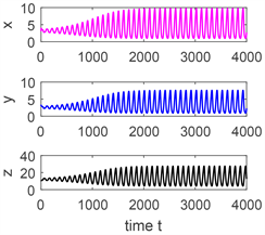
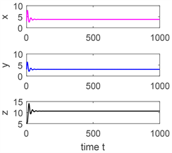
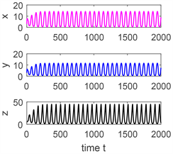
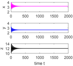
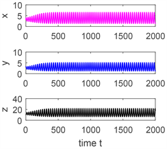
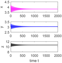
从图1~图4的数值模拟可知,当时滞参数值小于临界值时,系统的正平衡点是局部渐近稳定的,当时滞参数值不断增大时,系统的稳定性会发生变化,而且当时滞参数值大于临界值时系统会出现稳定的周期解。从图5~图8的数值模拟可知,我们同样可以得到相同的结论,当固定一个时滞参数在系统稳定的区间内,当另一个时滞参数值小于临界值时,系统的正平衡点是局部渐近稳定的,而当另一个时滞参数值不断增大时,系统的稳定性会发生变化,当它大于临界值时系统仍会出现稳定的周期解。
 (a)
(a)
 (b)
(b)
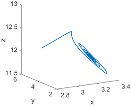
Figure 1. (a) Time series; (b) Phase portrait, the initial value is (3, 3, 10), when ,
, 
图1. (a) 当 ,
, ,初始值为(3, 3, 10)时,系统(1)的时间序列图;(b) 对应系统(1)相图
 (a)
(a)
 (b)
(b)
Figure 2. (a) Time series; (b) Phase portrait, the initial value is (3, 3, 10), when ,
, 
图2. (a) 当 ,
, ,初始值为(3, 3, 10)时,系统(1)的时间序列图;(b) 对应系统(1)相图
 (a)
(a)  (b)
(b)
Figure 3. (a) Time series; (b) Phase portrait, the initial value is (3, 3, 5), when ,
, 
图3. (a) 当 ,
, ,初始值为(3, 3, 5)时,系统(1)的时间序列图;(b) 对应系统(1)相图
 (a)
(a)
 (b)
(b)
Figure 4. (a) Time series; (b) Phase portrait, the initial value is (3, 3, 5), when ,
, 
图4. (a) 当 ,
, ,初始值为(3, 3, 5)时,系统(1)的时间序列图;(b) 对应系统(1)相图
 (a)
(a) 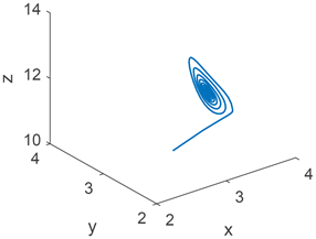 (b)
(b)
Figure 5. (a) Time series; (b) Phase portrait, the initial value is (3, 3, 10), when ,
, 
图5. (a) 当 ,
, ,初始值为(3, 3, 10)时,系统(1)的时间序列图;(b)对应系统(1)相图
 (a)
(a)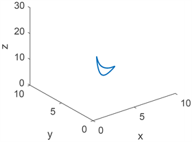 (b)
(b)
Figure 6. (a) Time series; (b) Phase portrait, the initial value is (3, 3, 10), when ,
, 
图6. (a) 当 ,
, ,初始值为(3, 3, 10)时,系统(1)的时间序列图;(b)对应系统(1)相图
 (a)
(a) (b)
(b)
Figure 7. (a) Time series; (b) Phase portrait, the initial value is (3, 3, 5), when ,
, 
图7. (a) 当 ,
, ,初始值为(3, 3, 5)时,系统(1)的时间序列图;(b) 对应系统(1)相图
 (a)
(a)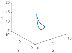 (b)
(b)
Figure 8. (a) Time series; (b) Phase portrait, the initial value is (3, 3, 5), when ,
, 
图8. (a) 当 ,
, ,初始值为(3, 3, 5)时,系统(1)的时间序列图;(b) 对应系统(1)相图
 (a)
(a) 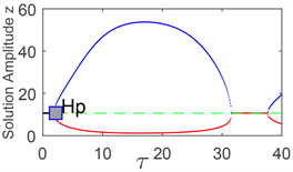 (b)
(b)
Figure 9. (a) Bifurcation diagram with  and z, the initial value is (3, 3, 5), when
 ; (b) Bifurcation diagram with
  and z, the initial value is (3, 3, 10), when
图9. (a) 将 作为一个参数,
 ,初始值为(3, 3, 5)时,模型(1)的Hopf分支图;(b) 当
 作为一个参数,
 ,初始值为(3, 3, 10)时,模型(1)的Hopf分支图
从图9的数值模拟可知,当固定一个时滞参数在系统的稳定区间内,改变另一个时滞参数的值时,系统的稳定性会发生改变,而且当参数值与临界值相等时系统会出现Hopf分支。
4. 结论
本文建立了一类具有双时滞效应的氮–磷–浮游植物动力学新模型,以此为基础对模型的相关动力学性质进行了数学分析与理论推导,解析出模型正平衡点具有局部渐近稳定性和发生Hopf分支的阈值条件,给出一些理论结果,同时模拟仿真出营养及浮游植物密度和Hopf分岔的动态演化过程。本论文的研究结果有助于深入理解时滞效应对海洋生态系统的影响,对预防和控制水体的富营养化具有一定的指导意义。
基金项目
国家自然科学基金面上项目(31570364)。
文章引用
赵潘. 一类具有双时滞效应的氮–磷–浮游植物模型的动力学研究
Dynamic Analysis of a Nitrogen-Phosphorus-Plankton Model with Two Time Delays[J]. 应用数学进展, 2018, 07(08): 1105-1118. https://doi.org/10.12677/AAM.2018.78128
参考文献
- 1. Dai, C. Zhao, M. and Yu, H. (2016) Dynamics Induced by Delay in a Nutrient-Phytoplankton Model with Diffusion. Ecological Complexity, 26, 29-36. https://doi.org/10.1016/j.ecocom.2016.03.001
- 2. Song, X. and Chen, L. (2001) Optimal Harvesting and Stability for a Two-Species Competitive System with Stage Structure. Mathematical Biosciences, 170, 173-186. https://doi.org/10.1016/S0025-5564(00)00068-7
- 3. Ruan, S. and Wei, J. (2003) On the Zeros of Transcendental Functions with Applications to Stability of Delay Differential Equations with Two Delays. Dynamics of Continuous, Discrete and Impulsive Systems Series A: Mathematical Analysis, 10, 863-874.
- 4. Laukkanen, M. and Huhtala, A. (2008) Optimal Management of a EUTROPHIED COASTAL ECOSYStem: Balancing agricultural and Municipal Abatement Measures. Environmental and Resource Economics, 39, 139-159. https://doi.org/10.1007/s10640-007-9099-2
- 5. Ruan, S. (1995) The Effect of Delays on Stability and Persistence in Plankton Models. Nonlinear Analysis, 24, 575-585. https://doi.org/10.1016/0362-546X(95)93092-I
- 6. Qin, B. (2009) Lake Eutrophication: Control Countermeasures and Recycling Exploitation. Ecological Engineering, 35, 1569-1573. https://doi.org/10.1016/j.ecoleng.2009.04.003
- 7. Reigada, R., Hillary, R.M., Bees, M.A., Sancho, J.M. and Sagues, F. (2003) Plankton Blooms Induced by Turbulent Flows. Proceedings of the Royal Society B: Biological Sciences, 270, 875-880. https://doi.org/10.1098/rspb.2002.2298
- 8. Gourley, S. A. and Ruan, S. (2003) Spatio-Temporal Delays in a Nutrient-Plankton Model on a Finite Domain: Linear Stability and Bifurcations. Applied Mathematics and Computation, 145, 391-412. https://doi.org/10.1016/S0096-3003(02)00494-0
- 9. Zhao, M., Yu, H. and Zhu, J. (2009) Effects of a Population Floor on the Persistence of Chaos in a Mutual Interference Host-Parasitoid Model. Chaos, Solitons and Fractals, 42, 1245-1250. https://doi.org/10.1016/j.chaos.2009.03.027
- 10. Yu, H., Zhao, M. and Agarwal, R.P. (2014) Stability and Dynamics Analysis of Time Delayed Eutrophication Ecological Model Based upon the Zeya Reservoir. Mathematics and Computers in Simulation, 97, 53-67. https://doi.org/10.1016/j.matcom.2013.06.008
- 11. Mei, L. and Zhang, X. (2012) Existence and Nonexistence of Positive Steady States in Multi-Species Phytoplankton Dynamics. Journal of Differential Equations, 253, 2025-2063. https://doi.org/10.1016/j.jde.2012.06.011
- 12. Wang, Y., Jiang, W. and Wang, H. (2013) Stability and Global Hopf Bifurcation in Toxic Phytoplankton-Zooplankton Model with Delay and Selective Harvesting. Nonlinear Dynamics, 73, 881-896. https://doi.org/10.1007/s11071-013-0839-2
- 13. Wang, B., Zhao, M., Dai, C., Yu, H., Wang, N. and Wang, P. (2016) Dynamics Analysis of a Nutrient-Plankton Model with a Time Delay. Discrete Dynamics in Nature and Society, 2016, Article ID: 9797624. https://doi.org/10.1155/2016/9797624
- 14. He, X. and Ruan, S. (1998) Global Stability in Chemostat-Type Plankton Models with Delayed Nutrient Recycling. Journal of Mathematical Biology, 37, 253-271. https://doi.org/10.1007/s002850050128
- 15. Song, Y., Peng, Y. and Wei, J. (2008) Bifurcations for a Predator-Prey System with Two Delays. Journal of Mathematical Analysis and Applications, 337, 466-479. https://doi.org/10.1016/j.jmaa.2007.04.001
- 16. Tripathi, J., Tyagi, S. and Abbas, S. (2015) Global Analysis of a Delayed Density Dependent Predator-Prey Model with Crowley-Martin Functional Response. Communications in Nonlinear Science and Numerical Simulation, 30, 45-69.
- 17. Li, L. and Liu, Z. (2010) Global Stability and Hopf Bifurcation of a Plankton Model with Time Delay. Nonlinear Analysis-Theory Methods & Applications, 72, 1737-1745. https://doi.org/10.1016/j.na.2009.09.014
- 18. Martin, A. and Ruan, S. (2001) Predator-Prey Models with Delay and Prey Harvesting. Journal of Mathematical Biology, 43, 247-267. https://doi.org/10.1007/s002850100095
- 19. Shi, Q., Shi, J. and Song, Y. (2017) Hopf Bifurcation in a Reaction-Diffusion Equation with Distributed Delay and Dirichlet Boundary Condition. Journal of Differential Equations, 263, 6537-6575. https://doi.org/10.1016/j.jde.2017.07.024
- 20. Shi, R. and Yu, J. (2017) Hopf Bifurcation Analysis of Two Zooplank-ton-Phytoplankton Model with Two Delays. Chaos Solution & Fractals, 100, 62-73. https://doi.org/10.1016/j.chaos.2017.04.044
- 21. Deng, Y., Zhao, M., Yu, H. and Wang, Y. (2015) Dynamical Analysis of a Nitrogen-Phosphorus-Phytoplankton Model. Discrete Dynamics in Nature and Society, 2015, Article ID: 823026.
- 22. Liu, J. (2015) Hopf Bifurcation Analysis for an SIRS Epidemic Model with Logistic Growth and Delays. Journal of Applied Mathematics & Com-puting, 50, 557-576.