Advances in Applied Mathematics
Vol.
10
No.
09
(
2021
), Article ID:
45273
,
16
pages
10.12677/AAM.2021.109320
捕食者患病的捕食–食饵模型的定性分析
李敏,卢旸*
东北石油大学数学与统计学院应用数学系,黑龙江 大庆

收稿日期:2021年8月14日;录用日期:2021年9月6日;发布日期:2021年9月17日

摘要
本文研究了捕食者患病的捕食–食饵模型,文中假设疾病仅在捕食者之间流行,其中易感捕食者和患病捕食者都具有捕获食饵的能力。本文首先运用极限理论以及构造Lyapunov函数的方法分别得到了各个边界平衡点的全局稳定性;其次运用一致持久生存理论得到了患病捕食者一致持久生存的充分条件。最后,运用数值模拟验证并补充了定性理论分析的结果。
关键词
捕食–食饵模型,全局稳定性,捕食者患病,一致持久性,定性分析

Qualitative Analysis of Predator-Prey Model with Infected Disease in Predator
Min Li, Yang Lu*
Department of Applied Mathematics, College of Mathematics and Statistics, Northeast Petroleum University, Daqing Heilongjiang

Received: Aug. 14th, 2021; accepted: Sep. 6th, 2021; published: Sep. 17th, 2021

ABSTRACT
In this paper, we study a predator-prey model with infected disease for predator. It is assumed that the disease only spreads among predators, both susceptible predators and infected predators have the ability to catch preys. Firstly, the global stability of each boundary equilibrium point is obtained by using the limit theory and the method of constructing the Lyapunov function. Secondly, we get the sufficient conditions of uniform persistence for the infected predator by using the uniform persistence theory. Finally, numerical simulation verifies and complements the results of qualitative theoretical analysis.
Keywords:Predator-Prey Model, Global Stability, Infected Predator, Uniform Persistence, Qualitative Analysis

Copyright © 2021 by author(s) and Hans Publishers Inc.
This work is licensed under the Creative Commons Attribution International License (CC BY 4.0).
http://creativecommons.org/licenses/by/4.0/


1. 引言
现实世界中,任何生物种群都处在某一群落中并与其它的种群存在着一定的联系,比如:依赖关系、竞争关系、捕食关系等。而捕食-食饵关系不仅是种群生态学中十分重要的研究对象,也是种群动力学研究中的一个有趣的课题,近几年来引起了许多专家和学者的广泛关注 [1] - [7]。
由于生物种群中流行的传染病会影响到种群的数量,因此对生态传染病模型的研究也日渐丰富 [8] - [14]。2005年,张江山 [15] 等人对捕食者患病的生态–流行病模型进行了定性分析,讨论了解的有界性并得到了平衡点局部渐近稳定的充分条件。Liu [16] 等人研究了一类具有非线性发病率的随机传染病模型,建立了一个由基本再生数
确定的阈值动态,结果表明
时疾病可以被根除,
时疾病会继续流行。2018年,卢旸 [17] 等人研究了食饵患病的非自治捕食–食饵模型:
其中,
表示食饵种群的补充率;
表示易感食饵的种群密度;
表示患病食饵的种群密度;
表示捕食者种群的密度;
表示患病食饵的死亡率;
表示易感食饵的自然死亡率(对任意
, );
为疾病发生率;
为捕食者对易感食饵的捕获率;
为捕食者对患病食饵的捕获率;
为捕食者捕获易感食饵后对其营养的转化率;
表示捕食者捕获患病食饵后对其营养的转化率;
表示捕食者的种内竞争率。运用比较原理得到了模型的一致持久性,此外还得到了患病食饵一致持久和灭绝的充分条件。
2. 模型的建立
由于在文献 [17] 中仅考虑的是食饵患病,并未考虑到捕食者患病这一因素,然而自然界中捕食者也会受到疾病的困扰,从而本文中就捕食者患病这一情形讨论了捕食者患病的捕食–食饵模型。文中考虑了两类种群:食饵种群
和捕食者种群
,在给出模型之前,首先做如下假设:
(1) 当食饵种群中无疾病传播时,食饵种群的内禀增长率为r,环境容纳量为K,数学上的描述为
。
(2) 假设疾病仅感染捕食者种群,则捕食者种群将划分为两类:易感捕食者种群
和患病捕食者种群
,则捕食者种群在任意t时刻的密度为
。
(3) 假设疾病不会通过垂直传播的方式由生病的母亲传染给孩子,并且患病捕食者不会自然恢复,或者自然免疫。假定发生率为双线性形式的
,其中
是平均接触感染概率。
(4) 易感捕食者和患病捕食者同时捕获食饵,用
分别表示易感捕食者
和患病捕食者
对食饵的捕获概率 [18];由于易感捕食者
比患病捕食者
的捕获能力更强 [19],故假设
。
(5)
表示食饵的自然死亡率,且
。
和
分别表示易感捕食者和患病捕食者的死亡率,由于捕食者患有疾病,故
, 和
分别表示易感捕食者和患病捕食者捕获食饵后的营养转化率且
。
基于上述假设,捕食者患病的捕食–食饵模型如下:
(1)
3. 准备工作
考虑到生物学意义,模型(1)的正向不变集为
。
模型解的有界性
命题3.1 模型(1)中所有满足初始条件
的解是正的且有界的。
证明 令
为模型(1)的任意解,且
,由
从而:
令:
从而,计算函数
沿着模型(1)的正解的全导数,可得:
令
,则:
由
,则存在正常数B和T使得当
时,
从而:
从而,模型(1)的解
为一致有界的。
4. 模型(1)的边界平衡点的稳定性
模型(1)的任意平衡点
满足:
可知模型(1)存在平衡点:
当
时,存在平衡点:
由模型假设可知当:
(2)
时,模型(1)还存在边界平衡点
和
:
此外模型(1)还有正平衡点
:
其中
设
为模型(1)的任意平衡点,则模型(1)在平衡点处的线性化矩阵为:
定理4.1 模型(1)在平衡点
处的线性化矩阵为:
则矩阵
对应的特征方程为:
从而特征根为:
当
时,所有特征根为负实根,从而
是不稳定的。
定理4.2 若模型(1)满足条件:
(3)
则模型(1)的平衡点
是全局渐近稳定的。
证明:模型(1)在平衡点
处的线性化矩阵为:
则矩阵
对应的特征方程为:
从而特征根为:
当模型(1)满足条件(3)时,由模型假设可得:
成立,从而所有特征根均具有负实部,平衡点
是局部渐近稳定的。
由模型(1)的第一个方程可得
,从而对于充分小的
,存在
使得当
时,
成立,将此不等式替换到模型(1)的第二个方程中,则当
时,
(4)
将不等式(4)两端同时积分可得:
当满足条件(3)时,对充分小的
,有
成立,因此,当
时,可得:
(5)
从而,存在正常数
,使得当
时,
成立。由模型(1)的第三个方程可得:
(6)
将不等式(6)两端积分,可得:
从而,由模型假设及条件(3),对充分小的
时,有
成立,从而当
时,可得:
(7)
由模型(1),式(5),式(7)可得
,则平衡点
是全局渐近稳定的。
定理4.3 如果模型(1)满足条件(2),且
(8)
成立,则边界平衡点
是全局渐近稳定的。其中
为患病捕食者
的净再生数 [20]。
证明:模型(1)在平衡点
处的线性化矩阵为:
则矩阵
对应的特征方程为:
其中
令
的两个特征根分别为
,由韦达定理及条件(2)可得:
因此可知
有两个负实部的特征根。
再由条件(8)可得:
从而平衡点
是局部渐近稳定的。
下面证明
的全局渐近稳定性。
定义函数
, 以及Lyapunov函数:
计算函数
沿着模型(1)的正解的全导数,则:
(9)
注意到由
为模型(1)的平衡点,从而:
因此由(9)式,可得:
由于平衡点
,以及条件(8)可得:
又因为模型假设(5)中
,从而
。由文献 [21] 中的定理5.3.1,可以证明
,
当且仅当
。故由Lyapunov-LaSalle不变集原理 [21],模型(1)的边界平衡点
是全局渐近稳定的。
定理4.4 (i) 若模型(1)满足条件(2),且
(10)
则边界平衡点
是全局渐近稳定的。其中
为健康捕食者
的净再生数 [20]。
(ii) 若模型(1)满足条件(2),(3),(8),则患病捕食者
是一致持久的。即存在常数
,使得:
证明:(i) 模型(1)在平衡点
处的线性化矩阵为:
则矩阵
对应的特征方程为:
其中
令
的两个特征根分别为
,由韦达定理及条件(2)可得:
从而可得
有两个负实部的特征根。
由条件(10),可得:
从而平衡点
是局部渐近稳定的。
下面证明
的全局渐近稳定性。
定义函数
, 以及Lyapunov函数:
计算函数
沿着模型(1)的正解的全导数,则:
(11)
由于
为模型(1)的平衡点,可得:
因此由(11)式,可得:
由于
,从而:
当
时,且由条件(10),可得
,由文献 [21] 中的定理5.3.1,可以证明
,当
且仅当
。故由Lyapunov-LaSalle不变集原理 [21],模型(1)的边界平衡点
是全局渐近稳定的。
下证(ii) 由文献( [22],定理1.3.2),令
为从
到
的连续函数映射空间。定义:
,
显然,
是相对于X的开集。定义T是基于X的连续半流,即对于任意的
, 为基于X的
-半群,且此半群满足:
由
和
的定义以及命题3.1,可得存在常数
使得
对于
是紧的,且
在X中最终一致有界。令
为轨道
的
极限集,定义
是特殊不变集,此不变集为:
.
为得到
极限集中的所有元素,首先需要讨论模型(1)基于
的动力学性态。当
, 时,模型(1)可以退化为下面的模型:
(12)
经过简单计算可知,模型(12)有三个平衡点:
,,
其中
不稳定;由条件(3),
是稳定的;由条件(2)和条件(8),
是稳定的。从而
是非循环的,由模型(1)可得
,且
中的流满足孤立非循环。
下面证明
, 和
对于
是一致弱排斥的。
步骤1。 首先证明
。如若结论不成立,则
,即存在正解
满足
。则对于充分小的正常数
满足
,存在正常
数
使得当
时,可得:
,,
成立。由模型(1)的第一个方程,可得:
因此,由比较原理和
的任意性,可得:
这与
时,
矛盾。从而,
。
步骤2。 接着证明
。如若结论不成立,则
,即存在模型(1)的正解
使得:
对于与步骤1中相同的
,存在正常数
,使得当
时,可得:
,,
由模型(1)的第三个方程,当
时,可得:
考虑方程:
(13)
由式(13)及比较原理,当
时,
。由条件(3),即
时,可得
,这与
时
矛盾。从而
。
步骤3。 最后运用类似的方法证明
。如若结论不成立,则
,即存在模型(1)的正解
使得:
对于与步骤2中相同的
,存在正常数
,使得当
时:
,,
由模型(1)的第三个方程,当
时:
考虑辅助方程:
(14)
由式(14)及比较原理,当
时,
。由条件(3),即
时,可得
,这与
时
矛盾。从而
。
上面的结论显示了在最大值范数意义下,下列不等式:
成立,故
对于
是一致弱排斥的。
从而,根据[22,定理1.3.2],存在常数
使得对于模型(1)的全部解有
,因此患病
捕食者一致持久生存。
5. 数值模拟
为验证并补充文中定性理论分析的结果,运用MATLAB软件进行了数值模拟。通过数值模拟可直观的显示出食饵
、易感捕食者
以及患病捕食者
的种群密度随时间变化的规律。
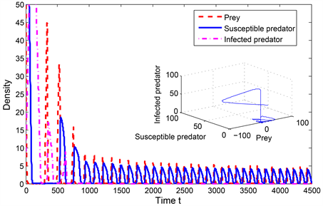
图1(a),图1(b)分别展示了模型(1)中边界平衡点
的全局渐近稳定性,疾病消除,易感捕食者与食饵共存的状态,参数选取如下:
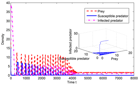
图2(a)~(c)分别展示了模型(1)中边界平衡点
的全局渐近稳定性,患病捕食者与食饵共存的状态,参数选取如下:
 (a)
(a)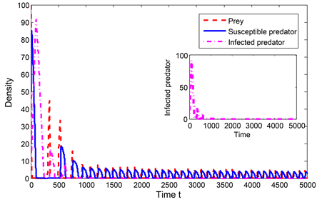 (b)
(b)
Figure 1. Global asymptotic stability of
with
图1. 当
时
的全局渐近稳定性
 (a)
(a)
 (b)
(b)
 (c)
(c)
Figure 2. Global asymptotic stability of
with
图2. 当
时
的全局渐近稳定性
 (a)
(a) (b)
(b)
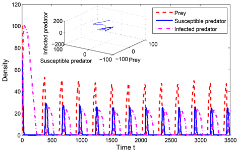
Figure 3. Global asymptotic stability of
图3.
的全局渐近稳定性
图3(a),图3(b)分别展示了模型(1)中正平衡点
的全局渐近稳定性,捕食者与食饵共存的状态,参数选取如下:
在本文定理4.3和定理4.4中,分别定义了易感捕食者
以及患病捕食者
的净再生数 [20],从而数值模拟图1和图2分别显示了当易感捕食者
以及患病捕食者
的净再生数分别小于1时,边界平衡点
和
的全局稳定性。
6. 结论
本文,提出了一个捕食者患病的捕食–食饵模型。文中假设易感捕食者和患病捕食者都具有捕获食饵的能力,食饵的自然增长率为Logistic型增长率。由于易感捕食者较患病捕食者的捕获能力更强,行动力更迅速,从而在模型假设的部分,本文分别就易感捕食者和患病捕食者对食饵的捕获率、捕食者自身的自然死亡率等做了相应的合理假设。在本文的主要内容部分通过运用渐近系统理论以及构造Lyapunov函数的方法分别获得了
和
的全局渐近稳定性,在给出
和
平衡点全局渐近稳定性的条件时,定义了易感捕食者和患病捕食者的净再生数,从而得出当
时
全局渐近稳定,而当
时
全局渐近稳定的结论。此外,本文运用一致持久生存理论得到了患病捕食者一致持久生存的充分条件。数值模拟图1,图2不仅验证了
的全局渐近稳定性,也显示了当易感捕食者
以及患病捕食者
的净再生数分别小于1时,边界平衡点
和
的全局稳定性。图3补充了正平衡点
的全局渐近稳定性。
在本文中,并未就正平衡点的全局稳定性给予定性理论的分析,也未讨论患病捕食者的灭绝性问题,这些都有待于将来去研究解决。
致谢
在此特别感谢东北石油大学校引导性基金项目(项目代码:2018YDL-04)以及东北石油大学–人才引进科研启动经费资助项目的支持(项目代码:1305021838)。
文章引用
李 敏,卢 旸. 捕食者患病的捕食–食饵模型的定性分析
Qualitative Analysis of Predator-Prey Model with Infected Disease in Predator[J]. 应用数学进展, 2021, 10(09): 3059-3074. https://doi.org/10.12677/AAM.2021.109320
参考文献
- 1. Briggs, C.J. and Hoopes, M.F. (2004) Stabilizing Effects in Spatial Parasitoid-Host and Predator-Prey Models: A Review. Theoretical Population Biology, 65, 299-315. https://doi.org/10.1016/j.tpb.2003.11.001
- 2. Wan, A., Song, Z. and Zheng, L. (2016) Patterned Solutions of a Homogenous Diffusive Predator-Prey System of Holling Type-Ⅲ. Acta Mathematicae Applicatae Sinica, 32, 1073-1086. https://doi.org/10.1007/s10255-016-0628-z
- 3. Liu, G. and Wang, Y. (2017) Stochastic Spatiotemporal Diffusive Predator-Prey Systems. Communications on Pure & Applied Analysis, 17, 67-84. https://doi.org/10.3934/cpaa.2018005
- 4. Yang, W., Wu, J. and Nie, H. (2015) Some Uniqueness and Multiplicity Results for a Predator-Prey Dynamics with a Nonlinear Growth Rate. Communications on Pure & Applied Analysis, 14, 1183-1204.
https://doi.org/10.3934/cpaa.2015.14.1183
- 5. Kant, S. and Kumar, V. (2017) Dynamics of a Prey-Predator System with Infection in Prey. Electronic Journal of Differential Equations, 2017, 1-27.
https://schlr.cnki.net/Detail/index/SJDJLAST/SJDJ9B85AA35DF4627444E49E912F78FAF4D
- 6. Jiang, Z., Wang, H. and Wang, H. (2010) Global Periodic Solutions in a Delayed Predator-Prey System with Holling II Functional Response. Kyungpook Mathematical Journal, 50, 255-266. https://doi.org/10.5666/KMJ.2010.50.2.255
- 7. Letetia, A. (2017) Analysis of a Predator-Prey Model: A Deterministic and Stochastic Approach. Journal of Biometrics & Biostatistics, 8, 1-9.
- 8. Ruan, S. and Wang, W. (2003) Dynamical Behavior of an Epidemic Model with a Nonlinear Incidence Rate. Journal of Differential Equations, 188, 135-163. https://doi.org/10.1016/S0022-0396(02)00089-X
- 9. Fan, M., Li, M. and Wang, K. (2001) Global Stability of an SEIS Epidemic Model with Recruitment and a Varying Total Population Size. Mathematical Biosciences, 170, 199-208. https://doi.org/10.1016/S0025-5564(00)00067-5
- 10. Zhang, J., Li, J.and Ma, Z. (2004) Global Analysis of SIR Epidemic Models with Population Size Dependent Contact Rate. Chinese Journal of Engineering Mathematics, 21, 259-267.
- 11. Wang, W. (2002) Global Behavior of an SEIRS Epidemic Model with Time Delays. Applied Mathematics Letters, 15, 423-428. https://doi.org/10.1016/S0893-9659(01)00153-7
- 12. Li, M., Smith, H. and Wang, L. (2001) Global Dynamics of an SEIR Epidemic Model with Vertical Transmission. SIAM Journal on Applied Mathematics, 62, 58-69. https://www.jstor.org/stable/3061896https://doi.org/10.1137/S0036139999359860
- 13. Meng, X., Chen, L. and Cheng, H. (2007) Two Profitless Delays for the SEIRS Epidemic Disease Model with Nonlinear Incidence and Pulse Vaccination. Applied Mathematics and Computation, 186, 516-529.
https://doi.org/10.1016/j.amc.2006.07.124
- 14. Wang, L. and Wu, X. (2018) Stability and Hopf Bifurcation for an SEIR Epidemic Model with Delay. Advances in the Theory of Nonlinear Analysis and Its Applications, 2, 113-127. https://doi.org/10.31197/atnaa.380970
- 15. 张江山, 孙树林. 捕食者有病的生态-流行病模型的分析[J]. 生物数学学报, 2005(2): 157-164.
- 16. Li, D., Liu, S. and Cui, J. (2017) Threshold Dynamics and Ergodicity of an SIRS Epidemic Model with Markovian Switching. Journal of Differential Equations, 263, 8873-8915. https://doi.org/10.1016/j.jde.2017.08.066
- 17. Lu, Y., Wang, X. and Liu, S. (2018) A Non-Autonomous Predator-Prey Model with Infected Prey. Discrete & Continuous Dynamical Systems B, 23, 3817-3836. https://doi.org/10.3934/dcdsb.2018082
- 18. Krivan, V. (1996) Optimal Foraging and Predator-Prey Dynamics. Theoretical Population Biology, 499, 265-290.
https://doi.org/10.1006/tpbi.1996.0014
- 19. Bethel, W. and Holmes, J. (1974) Correlation of Development of Altered Evasive Behavior in Gammarus Lacustris (Amphipoda) Harboring Cystacanths of Polymorphus Paradoxus (Acanthocephala) with the Infectivity to the Definitive Host. The Journal of Parasitology, 60, 272-274. https://doi.org/10.2307/3278463
- 20. Lu, X.J., Hui, L.L., Liu, S.Q. and Li, J. (2015) A Mathematical Model of HTLV-I Infection with Two Time Delays. Mathematical Biosciences and Engineering, 12, 431-449. https://doi.org/10.3934/mbe.2015.12.431
- 21. Hale, J. and Lunel, S. (1993) Introduction to Functional Differential Equations. Springer, New York.
https://doi.org/10.1007/978-1-4612-4342-7
- 22. Zhao, X. (2003) Dynamical Systems in Population Biology. Springer, New York.
https://doi.org/10.1007/978-0-387-21761-1
NOTES
*通讯作者。


 (a)
(a) (b)
(b) (a)
(a)
 (b)
(b)
 (c)
(c) (a)
(a) (b)
(b)