Advances in Applied Mathematics
Vol.
08
No.
12
(
2019
), Article ID:
33608
,
12
pages
10.12677/AAM.2019.812239
Soliton and Breather Solutions of Higher Order NLS-MB Equation in Erbium-Doped Fibers
Huihui Wang, Rui Guo*
College of Mathematics, Taiyuan University of Technology, Taiyuan Shanxi

Received: Dec. 2nd, 2019; accepted: Dec. 18th, 2019; published: Dec. 25th, 2019

ABSTRACT
In the nonlinear science, the soliton theory plays a significant role. The development of the soliton theory which has become the main instrument to solve nonlinear partial differential equations, has opened up a new direction for the study of nonlinear science. Specially, some nonlinear models involved in the fluid mechanics, the nonlinear optics, the plasma physics and other fields of natural science, can be described by the soliton equation. But with the development of optical pulse pressing technology, the perturbation of light pulses by some higher-order effects becomes prominent. In order to get more complex and obvious pulse phenomena, some soliton solutions and breather solutions of higher-order nonlinear Schrödinger and Maxwell-Bloch coupling equation are found by using the method of Darboux transformation. The results indicate that this approach is still simple and efficient for solving nonlinear evolution equation, and the breakthrough to higher order has been achieved at the same time. In the first section, we get the Lax pair of 4th order NLS-MB equation and find the corresponding darboux transformation. In the second section, the solutions of single- and double-solitons have been obtained and their figures are plotted. In the third section, single- and double-breathers solutions have been obtained and figures of the solutions are plotted. In the fourth section, the conclusions have been obtained.
Keywords:Darboux Transformation, NLS-MB Equation, Lax Pair, Soliton Solutions, Breather Solution

掺铒光纤中高阶NLS-MB方程的孤子解 与呼吸子解
王慧慧,郭睿*
太原理工大学数学学院,山西 太原

收稿日期:2019年12月2日;录用日期:2019年12月18日;发布日期:2019年12月25日

摘 要
在非线性科学中,孤子理论占有重要的地位,它的兴起开辟了非线性科学研究的新方向,成为求解非线性偏微分方程的主要手段。特别地,在流体力学、非线性光学、等离子物理等自然科学领域中涉及的非线性模型问题大部分都可以利用孤子方程来描述,但是随着光脉冲压榨技术的发展,一些高阶效应对光脉冲的扰动就会变得突出。为了得到更为复杂并明显的脉冲现象,本文运用Darboux变换的方法,求出了高阶非线性薛定谔(NLS)方程与Maxwell-Bloch系统耦合方程的孤子解及其呼吸子解。事实证明,在非线性发展方程的求解中,此方法非常简便易行,同时实现了向高阶迈进的突破。第一节,我们给出了4阶NLS-MB方程的Lax对并求出对应的达布变换。第二节,求出其单双孤子解并绘出解的图像。第三节,求出其单双呼吸子解并绘出解的图像。第四节,得出结论。
关键词 :Darboux变换法,NLS-MB方程,Lax对,孤子解,呼吸子解

Copyright © 2019 by author(s) and Hans Publishers Inc.
This work is licensed under the Creative Commons Attribution International License (CC BY).
http://creativecommons.org/licenses/by/4.0/


1. 引言
非线性发展方程目前已经应用到各个领域,它的飞速发展为化学、生物学、通信工程尤其是物理学的许多现象提供了重要的数学模型并予以简练而准确的描述,因而求解非线性问题一直是数学家和物理学家研究的重要课题。近年来已经有许多求解这些非线性发展方程的方法,例如反散射法、齐次平衡法、三角函数法、双函数法,最常用且最简便的方法为Darboux变换法。2004年,有人运用双曲函数法找到了变系数非线性方程的精确解 [1]。三年后,赵长海用双函数法获得NLS方程的多组新显式行波解,包括孤波解和周期解 [2]。2008年,王永杰等人运用齐次平衡法研究了描述阿尔芬波的导数NLS方程的精确解 [3]。2014年,毛春华用待定系数法求解了一类NLS方程的解 [4]。四阶NLS方程形式如下:
(1)
式中,q为关于时间变量t和空间变量x的实函数,它也代表着标准的非线性波理论。有时x和t在光波和水波中也是相互影响的 [5] [6]。在2014年,Adrian Ankiewicz,Nail Akhmediev求出了方程(1)的孤子解和呼吸子解 [7]。近几年,孤子脉冲动力学的研究在非线性光学中引起了人们广泛的兴趣。在光导纤维中存在两种类型的孤子。其中一种类型的传播通常由NLS方程所描述。另一种是相干脉冲,在两级共振介质中传播,通常由如下的MB方程所描述,
(2)
在某些情况下,这两种类型的孤子可能同时存在于一个纤维介质中,它的传播需要由NLS-MB系统来描述 [8]。本文在此基础上,将会给出高阶的NLS-MB方程的孤子解及其呼吸子解来得到更为明显且复杂的脉冲现象,耦合方程如下:
(3)
其中x是空间变量,t是时间变量。
2. Lax对及其达布变换
这一节中,我们将构建方程(3)的Lax对,进而构建其达布矩阵。Lax对具体形式如下
(4)
这里,
其中, 和 都是关于x和t的复杂函数,此时有
其中
(5)
(6)
(7)
这里
(8)
其中,
(9)
(10)
其中,
在我们的记号里,最后的矩阵, 为
(11)
如果 是实参数,则
通过直接计算,能够证明零曲率方程
(12)
一定能得到方程(3)。
接下来构建达布矩阵,令
(13)
这里I为单位矩阵,
(14)
这里,
我们能够证明如果 是当 时(4)的解,则 是对应 时(4)的解。
我们要求 必须满足
(15)
这里,
(16)
这里, , 和 与U和V有相同的形式,而 则被 所代替。通过直接计算,我们得到一次达布变换
(17)
(18)
(19)
3. 孤子解
这一节,我们将讨论方程(3)的孤子解,取种子解 。通过求解(4),我们能得到如下基本解
(20)
(21)
其中, 和 是实数。下面的工作将会通过达布变换求出单孤子解和双孤子解。
3.1. 单孤子解
将(20)和(21)两式带入(17),(18),(19)得到具体表达式,通过数学软件Mathematica,我们可以画出单孤子解图
 (a)
(a)
 (b)
(b)
 (c)
(c)
Figure 1. Evolution of the one-soliton solutions of Eqs.(3) via Expressions(17), (18), (19). The parameters adopted here are:
图1. 由式(17),(18),(19)表述的方程(3)的单孤子解的演化过程。参数取值为:
当种子解 时,单孤子解见图1,图1(a)和图1(c)是亮孤子,图1(b)是暗孤子。
3.2. 双孤子解
此小节在单孤子解的基础上,运用迭代的方法求出双孤子解。二次迭代后, ,其中
S和H同上不变,有
(22)
(23)
则二次达布变换为
(24)
(25)
(26)
综合以上,能够得到双孤子的图为
 (a)
(a)
 (b)
(b)
 (c)
(c)
Figure 2. Evolution of the two-soliton solutions of Equation (3) via Expressions (24), (25), (26). The parameters adopted here are:
图2. 由式(24),(25),(26)表述的方程(3)的双孤子解的演化过程。参数取值为:
从图2中可以看出,两个孤子的碰撞为弹性碰撞,碰撞之后的振幅和速度保持不变。
4. 呼吸子解
设系统(3)的非零连续波背景下的初始解为 。
这里 均为常数,将初始解带入原方程,得到如下关系:
(27)
(28)
求解(4)并且假设
(29)
我们得到
(30)
(31)
(32)
(33)
这里,
从上式我们容易得到 ,并且带入 和 的表达式中,可以得到具体值;另外, 和 也可以求出。通过计算:
(34)
这里,
其中,
假设 ,其中 为实数,则设有
(35)
又得
(36)
(37)
4.1. 单呼吸子解
根据(35),我们可以分如下几种情况:
情形4.1.1:当 ,此时 ,孤子解与x和t无关,因此讨论无意义。
情形4.1.2:当 ,得到 ,取适当的参数,可以画出单呼吸子解的图形如下:
 (a)
(a)
 (b)
(b)
 (c)
(c)
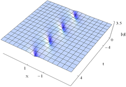
Figure 3. Evolution of the Akhmediev breathers. The parameters adopted here are:
图3. Akhmediev呼吸子解的演化。参数取为:
从图3中,我们得到,在连续波背景下,呼吸子解在空间上周期性传播,在时间上是非周期性传播的,因此我们获得了Akhmediev呼吸子解 [9] [10],另外,Akhmediev呼吸子解的传播能被视为调制不稳定过程 [11] [12],它是因为非线性和分散效应有相互作用,也被称为参变过程,在这个过程中,连续或类似连续波在微扰出现时,经受了振幅和相位的调制。图3(a)和(c)为明呼吸子,图3(b)为暗呼吸子。
情形4.1.3:当 ,得到 ,取适当的参数,可以画出单呼吸子解的图形如下:
 (a)
(a)
 (b)
(b)
 (c)
(c)
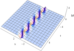
Figure 4. Evolution of the Ma breathers. The parameters adopted here are:
图4. Ma呼吸子解的演化过程。参数取值为:
从图4中,我们得到,在连续波背景下,呼吸子解在时间上周期性传播,在空间上是非周期性传播的,因此,在取到合适的参数下,我们获得了Ma呼吸子解 [13] [14],比较图4(a)~(c),图4(a)和图4(c)为明呼吸子,图4(b)为暗呼吸子。
4.2. 双呼吸子解
本节是在单呼吸子解的基础上利用达布变换的迭代求得双呼吸子解。具体为
 (38)
(38)
这里
 是Lax对(4)对应于谱参数
的另一个解,其中,
是Lax对(4)对应于谱参数
的另一个解,其中,
与 分别为 与 中 时的值,我们可以得到双呼吸子解的表达式为
(39)
(40)
(41)
假设 ,并且 ,则 和 满足(35),有
(42)
由上式,我们可以得出如下几种情况:
情形4.2.1:当 时, ,解与x和t无关,因此讨论无意义。
情形4.2.2:当 时, ,,,取适当参数,图形如下:
 (a)
(a)
 (b)
(b)
 (c)
(c)
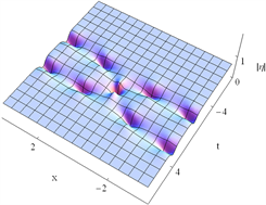
Figure 5. Evolutions of the parallel wave. The parameters adopted here are:
图5. 平行波的演化过程。参数取值为:
图5描述了两个振幅相同的波平行传播且相互不干涉,图5(a)和图5(c)为明呼吸子解,图5(b)为暗呼吸子解。
情形4.2.3:当 时, ,,,取适当的参数,可以画出双呼吸子解的图像如下:
 (a)
(a)
 (b)
(b)
 (c)
(c)
Figure 6. Evolutions of the two breathers. The parameters adopted here are:
图6. 双呼吸子解的演化。参数取值为:
图6显示的是双呼吸子解的传播特征,通过观察,两个波在相互碰撞时,振幅发生了变化,但碰撞之后,波形,波速和传播方向保持不变,换句话说,波的碰撞为弹性碰撞。
情形4.2.4:当 时, ,,,双呼吸子解如图所示:
 (a)
(a)
 (b)
(b)
 (c)
(c)
Figure 7. Evolutions of the Akhmediev breathers and Ma breathers. The parameters adopted here are:
图7. Akhmediev呼吸子解和Ma呼吸子解的演化。参数取值为:
图7显示了两种双呼吸子解在同一介质中共存的情形,Akhmediev呼吸子解在空间上周期性传播,Ma呼吸子解在时间上周期性传播,两种波传播是垂直的,并且在碰撞时不改变彼此的方向,速度和振幅。
5. 结论
本文主要讨论的是4阶NLS-MB方程,构建了此方程的Lax对和达布变换,并通过达布变换方法求得该方程的单孤子解和单呼吸子解,再经过达布变换的迭代,求得双孤子解和双呼吸子解。另外再经过Mathematic软件,画出孤子解和呼吸子解的图形,方便我们进行对其直观的描述。
文章引用
王慧慧,郭 睿. 掺铒光纤中高阶NLS-MB方程的孤子解与呼吸子解
Soliton and Breather Solutions of Higher Order NLS-MB Equation in Erbium-Doped Fibers[J]. 应用数学进展, 2019, 08(12): 2084-2095. https://doi.org/10.12677/AAM.2019.812239
参考文献
- 1. 石玉仁, 段文山, 吕克璞, 等. 变系数非线性Schrödinger方程的精确解[J]. 西北师范大学学报(自然科学版), 2004, 40(2): 27-30.
- 2. 赵长海. 非线性NLS方程的新显式精确行波解[J]. 南通大学学报(自然科学版), 2007, 6(3): 13-22.
- 3. 王永杰, 陶运超, 李向正. DNLS方程的精确解[J]. 河南科技大学学报(自然科学版), 2008, 29(1): 81-83.
- 4. 毛春华. NLS方程的一种新解[J]. 赤峰学院学报(自然科学版), 2014, 30(10): 7-8.
- 5. Agrawal, G.P. (2010) Nonlinear Fiber Optics (Optics and Photonics). 4th Edition, Academic Press, New York.
- 6. Osborne, A.R. (2010) Nonlinear Ocean Waves and the Inverse Scattering Transform. International Geophysics, 97, 49-68.
https://doi.org/10.1016/S0074-6142(10)97003-4 - 7. Ankiewicz, A. and Akhmediev, N. (2014) Higher-Order Integrable Evolution Equation and Its Soliton Solutions. Physics Letters A, 378, 358-361.
https://doi.org/10.1016/j.physleta.2013.11.031 - 8. Guo, R., Hao, H.Q. and Zhang, L.L. (2013) Bound Solitons and Breathers for the Generalized Coupled Nonlinear Schrödinger-Maxwell-Bloch System. Modern Physics Letters B, 27, Article ID: 1350130.
https://doi.org/10.1142/S0217984913501303 - 9. Xu, Z.Y., Li, L., Li, Z.H., et al. (2003) Modulation Instability and Solitons on a cw Background in an Potical Fiber with Higher-Order Effects. Physical Review E, 67, Article ID: 026603.
https://doi.org/10.1103/PhysRevE.67.026603 - 10. Akhmediev, N.N. and Korneev, V.I. (1986) Modulation Instability and Periodic Solutions of the Nonlinear Schrödinger Equation. Theoretical and Mathematical Physics, 69, 1089-1093.
https://doi.org/10.1007/BF01037866 - 11. Kamchatnov, A.M. (2000) Nonlinear Periodic Waves and Their Modulations. World Scientific Press, Hong Kong.
https://doi.org/10.1142/4513 - 12. Li, L., Li, Z.H., Li, S.Q., et al. (2004) Modulation Instability and Solitons on a cw Background in Inhomogeneous Optical Fiber Media. Optics Communications, 234, 169-176.
https://doi.org/10.1016/j.optcom.2004.02.022 - 13. Ma, Y.C. (1979) The Perturbed Plane-Wave Solutions of the Cubic Schrödinger Equation. Studies in Applied Mathematics, 60, 43-58.
https://doi.org/10.1002/sapm197960143 - 14. Guo, R. and Hao, H.Q. (2013) Breathers and Multi-Soliton Solutions for the Higher-Order Generalized Nonlinear Schrödinger Equation. Communications in Nonlinear Science and Numerical Simulation, 18, 2426-2435.
https://doi.org/10.1016/j.cnsns.2013.01.019