Advances in Applied Mathematics
Vol.
11
No.
07
(
2022
), Article ID:
53577
,
10
pages
10.12677/AAM.2022.117477
有限资源下杀虫剂具有残留作用的害虫综合 控制的数学模拟研究
唐玲碧,刘晓虎,刘兵*,李金洋
鞍山师范学院,数学与信息科学学院,辽宁 鞍山
收稿日期:2022年6月11日;录用日期:2022年7月6日;发布日期:2022年7月13日

摘要
本文考虑到杀虫剂的残留作用、喷洒前后对种群的作用方式的改变以及天敌资源的有限性,首先建立并系统地研究了资源有限下杀虫剂具有残留作用的固定时刻的害虫控制切换系统,分析关键参数对害虫灭绝阈值的影响;其次建立资源有限下依赖于害虫种群数量的状态害虫控制切换系统,通过数值模拟分析在规定的时间内影响杀虫剂的使用频率的因素。
关键词
害虫综合控制,局部渐近稳定性,全局吸引,资源有限,杀虫剂的残留作用

Mathematical Simulations of Integrated Pest Control with Pesticide Residues under Limited Resources
Lingbi Tang, Xiaohu Liu, Bing Liu*, Jinyang Li
School of Mathematics and Information Science, Anshan Normal University, Anshan Liaoning
Received: Jun. 11th, 2022; accepted: Jul. 6th, 2022; published: Jul. 13th, 2022

ABSTRACT
Considering the residual effect of pesticides, the change of the mode of action of the population before and after spraying pesticides and the limitation of natural enemy resources, firstly, a fixed-time pest control switching system with residual effect of pesticides under limited resources is established and systematically studied, and the influence of key parameters on the pest eradication threshold is analyzed. Secondly, a state pest control switching system that is dependent on the amount of pest populations under limited resources is established, and the factors that affect the frequency of pesticide use in the specified time are analyzed by numerical simulations.
Keywords:Integrated Pest Management, Local Asymptotic Stability, Global Attractiveness, Limited Resources, Residual Effects of Pesticides

Copyright © 2022 by author(s) and Hans Publishers Inc.
This work is licensed under the Creative Commons Attribution International License (CC BY 4.0).
http://creativecommons.org/licenses/by/4.0/


1. 引言
目前,害虫仍然是影响世界各国农业生产的主要危害之一。2019年草地贪夜蛾的入侵和2020年东非蝗灾,摧毁了数万公顷农田,对许多国家的农业生产造成了严重损害。已有很多学者利用脉冲动力系统来模拟固定时刻喷洒杀虫剂和释放天敌的过程,研究害虫的综合治理问题 [1] - [6]。但实际上,害虫控制的目的是控制害虫在经济危害水平之下,只有当害虫种群的密度达到经济阈值ET (Economic Threshold)时才实施害虫控制策略,可以利用状态依赖的脉冲动力系统来刻画,这方面的相关工作可以参阅文献 [7] [8] [9]。上述有关固定时刻和状态依赖的害虫控制模型都是假设杀虫剂瞬间、成比例杀死害虫和天敌的,并没有考虑到杀虫剂喷洒以后在相当长的时间里对害虫、天敌仍然持续起作用,在此背景下文献 [10] [11] [12] 引入杀虫剂作用函数,模拟杀虫剂对害虫的残留作用。上述文献均假设天敌是常数释放的,考虑到天敌资源的有限性,Li等在文献 [13] 中建立并研究了非线性脉冲控制的害虫控制模型,给出害虫灭绝周期解全局渐近稳定的条件。本文在上述工作的基础上,综合考虑杀虫剂的残留作用、喷洒前后对种群的作用方式的改变以及天敌资源的有限性,分别建立并研究固定时刻和状态依赖的害虫综合治理切换模型,分析主要参数对害虫控制和喷洒频率的影响。
2. 资源有限下固定时刻害虫综合治理模型的研究
2.1. 模型建立
文献 [2] 建立并研究了一个具有Ivlev型功能性反应函数等周期不同固定时刻喷洒杀虫剂和释放天敌的害虫综合治理模型,但是并没有考虑到杀虫剂的残留作用、喷洒前后对种群的作用方式的改变以及天敌资源有限性,基于此本文建立如下模型:
(2.1)
其中 , 分别表示在t时刻害虫和天敌的种群数量;a表示天敌对害虫的捕食效率,a表示天敌对害虫的捕食效率,函数 是Ivlev型功能反应函数;T是释放天敌的周期; 表示在每个周
期T内喷洒杀虫剂的时刻; 表示 时刻释放天敌的量, 为形状参数;这里
分别表示杀虫剂喷洒以后对害虫和天敌的作用, 分别为杀虫剂对害虫和天敌作用的杀死率; 分别为杀虫剂对害虫和天敌作用的衰减率。模型中其他参数生物意义同 [2]。
2.2. 系统(2.1)的动力学性质
对于子系统:
(2.2)
类似于 [13] 中定理2.2的证明,可得
定理2.1 如果 ,系统(2.2)存在一个全局渐近稳定的正T周期解 ,并且对模型(2.2)的任何解 都有:当 时, ,其中
(2.3)
这里
因此,由定理2.1知系统(2.2)存在害虫根除周期解 。
令
定理2.2 如果 ,系统(2.2)的害虫根除周期解 是局部渐近稳定的。
证明 设 是以 为初始值的系统(2.2)的解,则 的局部渐近稳定性可以通过对周期解附近小振幅摄动的解的动态行为来研究。令
则 可以写成如下形式
其中, ,并且 , 满足
因此
与 的表达式与后面的计算无关。在脉冲点 处,系统(2.1)的线性化矩阵如下:
从而得单值矩阵
经计算矩阵M的两个特征值分别为:
因此,由Floquet理论知,当 时,系统(2.1)的害虫根除周期解 是局部渐近稳定的。
令
其中
定理2.3 如果 ,系统(2.1)的害虫根除周期解 是全局吸引的。
证明 由 ,所以存在充分小的 ,使得
,
由系统(2.1)有
(2.4)
由定理2.1及脉冲微分方程比较定理知,当t充分大时, ,为方便起见,假设对所有 , 均成立,由系统(2.1)的第一个和第三个方程,不妨设
则有
当x足够小时, ,其中, ,因此积分
令
其中 ,因此当 时, ,此时,害虫种群趋于灭绝。在 上,有
因此,对 ,都存在一个正整数m,使得 时,
显然积分 有上界。又 ,如果
那么, ,即当 时, 。
下面我们证明 时, 。由上面可知, 时, 。为方便起见,假设对 , 均成立,从而
对上面两个不等式右端,考虑下面的微分方程
(2.5)
用与定理2.1相同的方法,系统(2.5)存在全局渐近稳定的周期解:
其中,
因此,当 时, 。所以,系统(2.2)的害虫根除周期解 是全局吸引的。
故当 时,令 ,则有
因此,当 时, 。所以,系统(2.2)的害虫根除周期解 是全局吸引的。
经过简单计算可以得到 ,因此有
定理2.4 如果 ,则系统(2.1)的害虫根除周期解 是全局渐近稳定的。
2.3. 主要参数对害虫根除阈值的影响
首先,考虑喷洒杀虫剂时刻和天敌释放量对害虫根除阈值 的影响。图1(a)和图1(b)分别表明阈值 关于T是单调增函数,关于天敌释放量 是单调减函数。这说明生物控制周期T的减小和天敌释放量的增加有利于害虫控制。其次,图2(a)和图2(b)分别给出 关于l和T的等高线, 和 的等高线,结果表明 分别是关于l的单调增加函数, 的单调减函数, 是单调增函数,因此,越早喷洒杀虫剂,杀虫剂对害虫杀死率越大,杀虫剂对天敌杀死率越小越有利于害虫控制。
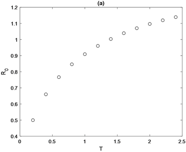
Figure 1. (a) Effects of biological control period T on threshold value R0, the parameter values are r = 0.8, k = 0.8, σ = 10, θ = 25, a = 0.5, D = 0.3, l = 0.7, δ2 = 0.2, σ = 10, m1 = 0.7, m2 = 0.5, δ1 = 0.5, T = 1; (b) Effect of released natural enemies amount σ on threshold value R0, the parameter values are r = 0.8, k = 0.8, σ = 10, θ = 5, a = 0.1, D = 0.15, l = 0.7, δ2 = 0.5, σ = 10, m1 = 0.5, m2 = 0.1, δ1 = 0.1, T = 2
图1. (a) 生物控制周期T对阈值R0的影响,参数取值为r = 0.8,k = 0.8,σ = 10,θ = 25,a = 0.5,D = 0.3,l = 0.7,δ2 = 0.2,σ = 10,m1 = 0.7,m2 = 0.5,δ1 = 0.5,T = 1;(b) 释放天敌数量σ对阈值R0的影响,参数取值为r = 0.8,k = 0.8,σ = 10,θ = 5,a = 0.1,D = 0.15,l = 0.7,δ2 = 0.5,σ = 10,m1 = 0.5,m2 = 0.1,δ1 = 0.1,T = 2
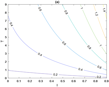
Figure 2. (a) Contour lines of R0 with respect to T and l, the parameter values are a = 0.2, r = 0.8, k = 0.8, σ = 9.5, θ = 2, D = 0.2, δ1 = 0.4, δ2 = 0.1, T = 3, l = 0.1, m1 = 0.4, m2 = 0.2; (b) Contour lines of R0 with respect to m1 and m2, the parameter values are a = 0.4, r = 0.8, k = 0.6, σ = 5, θ = 14, D = 0.4, δ1 = 0.5, δ2 = 0.3, T = 1, l = 0.4, m1 = 0.2, m2 = 0.1
图2. (a) R0关于T和l的等高线,参数取值为a = 0.2,r = 0.8,k = 0.8,σ = 9.5,θ = 2,D = 0.2,δ1 = 0.4,δ2 = 0.1,T = 3,l = 0.1,m1 = 0.4,m2 = 0.2;(b) R0关于m1和m2的等高线,参数取值为a = 0.4,r = 0.8,k = 0.6,σ = 5,θ = 14,D = 0.4,δ1 = 0.5,δ2 = 0.3,T = 1,l = 0.4,m1 = 0.2,m2 = 0.1
图1(a)同时表明阈值 关于T是单调增函数,因此存在临界值 ,当 时,害虫根除周期解是局部渐近稳定的(见图3(a));当 时,害虫种群最终会爆发(见图3(b))。
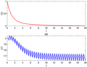
Figure 3. Time series graphs of pest population and natural enemy population of system (3.2), (a) T = 0.5, (b) T = 7, other parameters are a = 0.5, r = 0.6, k = 0.8, σ = 3, θ = 10, D = 0.3, δ1 = 0.4, δ2 = 0.6, l = 0.6, m1 = 0.2, m2 = 0.1, x0 = 1, y0 = 2
图3. 系统(3.2)害虫种群和天敌种群的时间序列图,(a) T = 0.5,(b) T = 7,其他参数取值为a = 0.5,r = 0.6,k = 0.8,σ = 3,θ = 10,D = 0.3,δ1 = 0.4,δ2 = 0.6,l = 0.6,m1 = 0.2,m2 = 0.1,x0 = 1,y0 = 2
3. 资源有限下状态依赖害虫综合治理模型的研究
使用杀虫剂能够有效控制害虫的暴发,但是杀虫剂的频繁使用会使害虫产生抗药性,而且对害虫的天敌也产生危害。所以,只有当害虫的种群数量达到ET时,才喷洒杀虫剂。假设害虫种群数量达到ET的时刻分别为 且 ,建立如下模型。
(3.1)
由于系统(3.1)的理论分析较为复杂,因此下面仅通过数值模拟分析影响杀虫剂喷洒频率的因素。设害虫和天敌的初始值分别为 ,。其他参数意义与系统(2.1)中的相同。
考虑 杀虫剂的喷洒频率,参数取值为 ,,,,,,,,,,,。在图4(a)中,取在图4(a)中,取 时,喷洒一次杀虫剂就可以控制害虫在ET之下。当害虫和天敌的初值分别为 、 和 时,从图4(b)、图4(c)和图4(d)中可以看出,三种不同初值状态下杀虫剂分别需要喷洒2次、3次、4次才能成功控制害虫。固定 ,当 变为 后,杀虫剂喷洒的次数由4次变为3次(见图4(e))。固定 ,改变周期令 ,此时不需要喷洒杀虫剂就可以使害虫种群小于ET (见图4(f))。上述结果表明,杀虫剂的喷洒频率依赖于害虫和天敌种群的初值、天敌释放量和天敌释放周期。
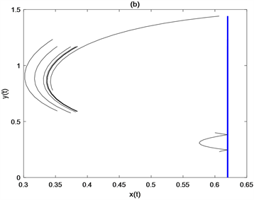
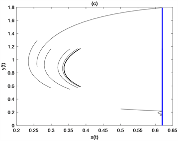
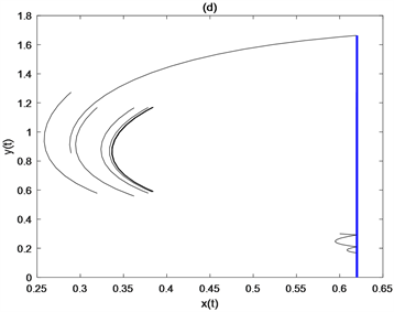
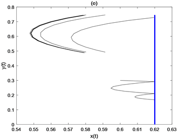
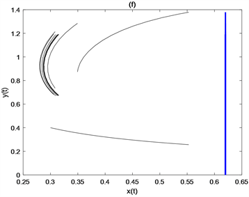
Figure 4. Effects of initial density of pest population and natural enemy population, release amount of natural enemy and release cycle of natural enemy on pesticide spraying frequency
图4. 害虫种群和天敌种群的初始密度、天敌释放量、释放天敌周期对杀虫剂使用次数的影响
4. 结论
本文首先建立了一个资源有限下杀虫剂具有残留的固定时刻害虫综合控制的切换模型。结果表明天敌资源有限情况下,害虫根除周期解局部渐近稳定性并不能保证其全局渐近稳定性。由于 ,所以只有当 时,害虫灭绝周期解是全局渐近稳定的。同时数值模拟分析表明缩短释放天敌周期,每周期内越早喷洒杀虫剂,增加天敌的释放量,增强杀虫剂对害虫的杀死率,减小杀虫剂对天敌的作用将有利于害虫控制。其次,为了避免频繁使用杀虫剂,考虑只有当害虫种群数量达到ET时才喷洒杀虫剂,建立了相应的状态依赖的害虫综合控制切换模型。结果表明,在规定时间内如果控制害虫在经济阈值之下,杀虫剂的使用频率依赖于害虫和天敌的初值、天敌的释放量和天敌释放的周期。本文所得结论可以为农业生产部门提供借鉴。
基金项目
国家自然科学基金项目(12171004),大学生创新创业项目(202110169054)。
文章引用
唐玲碧,刘晓虎,刘 兵,李金洋. 有限资源下杀虫剂具有残留作用的害虫综合控制的数学模拟研究
Mathematical Simulations of Integrated Pest Control with Pesticide Residues under Limited Resources[J]. 应用数学进展, 2022, 11(07): 4509-4518. https://doi.org/10.12677/AAM.2022.117477
参考文献
- 1. Gao, S.J., Luo, L., Yan, S.X. and Meng, X.Z. (2018) Dynamical Behavior of a Novel Impulsive Switching Model for HLB with Seasonal Fluctuations. Complexity, 2018, Article ID: 2953623. https://doi.org/10.1155/2018/2953623
- 2. Liu, B., Ying, Z. and Chen, L.S. (2004) The Dynamics of a Preda-tor-Prey Model with Ivlev’s Functional Response Concerning Integrated Pest Management. Acta Mathematicae Applica-tae Sinica, 20, 133-146. https://doi.org/10.1007/s10255-004-0156-0
- 3. Gao, S.J., Guo, J., Xu, Y., Tu, Y.B. and Zhu, H.P. (2021) Mod-eling and Dynamics of Physiological and Behavioral Resistance of Asian Citrus Psyllid. Mathematical Bioscience, 340, Article ID: 108674. https://doi.org/10.1016/j.mbs.2021.108674
- 4. Lan, G.J., Fu, Y.J., Wei, C.J. and Zhang, S.W. (2018) A Research of Pest Management SI Stochastic Model Concerning Spraying Pesticide and Releasing Natural Enemies. Communica-tions in Mathematical Biology and Neuroscience, 2018, 3648. http://scik.org/index.php/cmbn/article/view/3648
- 5. Liang, J.H., Tang, S.Y. and Cheke, R.A. (2016) Beverton-Holt Discrete Pest Management Models with Pulsed Chemical Control and Evolution of Pesticide Resistance. Communica-tions in Nonlinear Science and Numerical Simulation, 36, 327-341. https://doi.org/10.1016/j.cnsns.2015.12.014
- 6. Tian, Y., Tang, S.Y. and Cheke, R.A. (2019) Dynamic Complex-ity of a Predator-Prey Model for IPM with Nonlinear Impulsive Control Incorporating a Regulatory Factor for Predator Releases. Mathematical Modelling and Analysis, 24, 134-154. https://doi.org/10.3846/mma.2019.010
- 7. Tang, S.Y., Tang, B., Wang, A.L. and Xiao, Y.N. (2015) Holling II Predator-Prey Impulsive Semi-Dynamic Model with Com-plex Poincaré Map. Nonlinear Dynamics, 81, 1575-1596. https://doi.org/10.1007/s11071-015-2092-3
- 8. Zhang, Q.Q., Tang, B., Cheng, T.Y. and Tang, S.Y. (2020) Bifurcation Analysis of a Generalized Impulsive Kolmogorov Model with Applications to Pest and Disease Control. SIAM Journal on Applied Mathematics, 80, 1796-1819. https://doi.org/10.1137/19M1279320
- 9. Tang, S.Y., Li, C.T., Tang, B. and Wang, X. (2019) Global Dynamics of a Nonlinear State-Dependent Feedback Control Ecological Model with a Multiple-Hump Discrete Map. Communica-tions in Nonlinear Science and Numerical Simulation, 79, Article ID: 104900. https://doi.org/10.1016/j.cnsns.2019.104900
- 10. Tang, S.Y., Liang, J.H., Tan, Y.S. and Cheke, R.A. (2013) Threshold Conditions for Integrated Pest Management Models with Pesticides That Have Residual Effects. Journal of Mathematical Biology, 66, 1-35. https://doi.org/10.1007/s00285-011-0501-x
- 11. Kang, B.L., Liu, B. and Tao, F.M. (2018) An Integrated Pest Management Model with Dose Response Effect of Pesticides. Journal of Biological System, 26, 59-86. https://doi.org/10.1142/S0218339018500043
- 12. Liu, B., Tao, F.M., Kang, B.L. and Hu, G. (2021) Modelling the Effects of Pest Control with Development of Pesticide Resistance. Acta Mathematicae Applicatae Sinica, English Se-ries, 37, 109-125. https://doi.org/10.1007/s10255-021-0988-x
- 13. Li, C.T. and Tang, S.Y. (2018) Analyzing a Generalized Pest-Natural Enemy Model with Nonlinear Impulsive Control. Open Mathematics, 16, 1390-1411. https://doi.org/10.1515/math-2018-0114
NOTES
*通讯作者。