一类非自治随机互惠系统的渐近性态 Asymptotic Behavior of a Non-Autonomous Stochastic Mutualism System

doi:10.12677/PM.2019.94068

Pure Mathematics
Vol. 09 No. 04 ( 2019 ), Article ID: 30964 , 13 pages
10.12677/PM.2019.94068

Asymptotic Behavior of a Non-Autonomous Stochastic Mutualism System

Ao Guo, Xiaoquan Ding^*

●How to Cite this Article

School of Mathematics and Statistics, Henan University of Science and Technology, Luoyang Henan

Received: May 31^st, 2019; accepted: Jun. 10^th, 2019; published: Jun. 26^th, 2019

ABSTRACT

This paper is devoted to the asymptotic behavior of a non-autonomous stochastic mutualism system. Firstly, the existence and uniqueness of global positive solution to the system is established for any positive initial value. Then by using the comparison theorem for stochastic differential equations and Lyapunov functions, the sufficient conditions for the permanence, extinction, global attractivity, and existence of periodic solutions to the system are derived respectively. Finally, some numerical simulations are given to illustrate our theoretical results.

Keywords:Stochastic Mutualism System, Global Attractivity, Permanence, Extinction, Periodic Solution

一类非自治随机互惠系统的渐近性态

郭奥，丁孝全^*

河南科技大学数学与统计学院，河南洛阳

收稿日期：2019年5月31日；录用日期：2019年6月10日；发布日期：2019年6月26日

摘要

本文讨论一类非自治随机互惠系统的渐近性态。首先，对任意正初值，建立了系统全局正解的存在唯一性。接着，利用随机微分方程比较定理和Lyapunov函数，得到了系统的持续性、灭绝性、全局吸引性和周期解的存在性。最后，数值模拟验证了理论结果的合理性。

关键词 :随机互惠系统，全局吸引性，持续性，灭绝性，周期解

This work is licensed under the Creative Commons Attribution International License (CC BY).

http://creativecommons.org/licenses/by/4.0/

1. 引言

在自然界中，种群之间的互惠关系是非常普遍的，如传粉昆虫与开花植物、豆科植物与根瘤菌、海葵与小丑鱼等。许多学者对互惠种群模型进行了深入研究，并获得了丰富的研究成果 [1] [2] [3] [4] 。而现实世界中，种群的演化不可避免地受到环境噪声的影响，而且这些噪声是不容忽视的，更合理的种群模型应包括随机因素 [5] - [11] 。近年来，随机互惠模型受到学术界的广泛关注 [11] - [21] 。

2006年，Gravesa等人 [3] 提出以下互惠模型

${\begin{array}{l} \frac{d x_{1} (t)}{d t} = x_{1} (t) [r_{1} - b_{1} e^{- k_{1} x_{2} (t)} - c_{1} x_{1} (t)], \\ \frac{d x_{2} (t)}{d t} = x_{2} (t) [r_{2} - b_{2} e^{- k_{2} x_{1} (t)} - c_{2} x_{2} (t)], \end{array}$ (1.1)

其中 $x_{i} (t) (i = 1, 2)$ 是第i个种群在时刻t的种群密度； $r_{i}, b_{i}, c_{i}, k_{i}$ 为正常数，相应的生物意义见文献 [3] 。2009年，向等人 [4] 在系统(1.1)的基础上，考虑以下非自治互惠模型

${\begin{array}{l} \frac{d x_{1} (t)}{d t} = x_{1} (t) [r_{1} (t) - b_{1} (t) e^{- k_{1} (t) x_{2} (t)} - c_{1} (t) x_{1} (t)], \\ \frac{d x_{2} (t)}{d t} = x_{2} (t) [r_{2} (t) - b_{2} (t) e^{- k_{2} (t) x_{1} (t)} - c_{2} (t) x_{2} (t)], \end{array}$ (1.2)

建立了系统(1.2)的持续性、周期解的存在性和全局吸引性。2011年，为探讨随机扰动对系统(1.1)的影响，吕 [11] 考虑以下随机互惠模型

${\begin{matrix} d x_{1} (t) = x_{1} (t) [r_{1} - b_{1} e^{- k_{1} x_{2} (t)} - c_{1} x_{1} (t)] d t + σ_{1} x_{1} (t) d B_{1} (t), \\ d x_{2} (t) = x_{2} (t) [r_{2} - b_{2} e^{- k_{2} x_{1} (t)} - c_{2} x_{2} (t)] d t + σ_{2} x_{2} (t) d B_{2} (t), \end{matrix}$ (1.3)

给出了系统(1.3)的持续性、灭绝性和全局吸引性。

本文在文献 [3] [4] [11] 基础上，研究以下具有随机干扰的非自治互惠模型

${\begin{cases} d x_{1} (t) = x_{1} (t) [r_{1} (t) - b_{1} (t) e^{- k_{1} (t) x_{2} (t)} - c_{1} (t) x_{1} (t)] d t + σ_{1} (t) x_{1} (t) d B_{1} (t), \\ d x_{2} (t) = x_{2} (t) [r_{2} (t) - b_{2} (t) e^{- k_{2} (t) x_{1} (t)} - c_{2} (t) x_{2} (t)] d t + σ_{2} (t) x_{2} (t) d B_{2} (t), \end{cases}$ (1.4)

其中对 $r_{i} (t), b_{i} (t), k_{i} (t), c_{i} (t), σ_{i} (t) (i = 1, 2)$ 是连续函数，具有正的上、下界； ${(B_{1} (t), B_{2} (t))}^{T}$ 是定义在完备概率空间 $(Ω, F, {F}_{t \geq 0}, ℙ)$ 上的二维标准Brown运动。本文旨在利用随机微分方程理论 [22] [23] [24] [25] ，探讨系统(1.4)的全局正解的存在唯一性、持续性、灭绝性、全局吸引性和周期解的存在性。

为方便讨论，给出以下记号：

1) $R_{+}^{2} = {(x_{1}, x_{2}) : x_{1} > 0, x_{2} > 0}$ ；

2) 对 $[0, \infty)$ 上的有界函数f，定义 $\overset{⌣}{f} = \sup_{t \in [0, \infty)} f (t), \overset{⌢}{f} = \inf_{t \in [0, \infty)} f (t)$ ；

3) 给定 $θ > 0$ ，对 $[0, θ]$ 上的可积函数g，定义 ${〈 g 〉}_{θ} = \frac{1}{θ} \int_{0}^{θ} g (s) d s$ 。

2. 正解的存在唯一性

本节建立系统(1.4)的全局正解的存在唯一性，这是本文后续工作的基础。

定理2.1：对任意初值 $x (0) = {(x_{1} (0), x_{2} (0))}^{T} \in R_{+}^{2}$ ，系统(1.4)存在唯一的全局解 $x (t) = {(x_{1} (t), x_{2} (t))}^{T}$ ，并且该解以概率1停留在 $R_{+}^{2}$ 中。

证明：易知系统(1.4)的系数满足局部Lipschitz条件。因此，对于任意初值 $x (0) \in R_{+}^{2}$ ，系统(1.4)在区间 $[0, τ_{e})$ 上存在唯一的局部解 $x (t) = {(x_{1} (t), x_{2} (t))}^{T}$ ，其中 $τ_{e}$ 是爆破时刻。下面证明 $x (t)$ 是全局的，即证明 $τ_{e} = \infty$ 几乎必然成立。取充分大的正整数 $m_{0}$ ，使 $x_{1} (0) \in (\frac{1}{m_{0}}, m_{0})$ 和 $x_{2} (0) \in (\frac{1}{m_{0}}, m_{0})$ 。对任意正整数 $m > m_{0}$ ，定义停时：

$τ_{m} = \inf {t \in [0, τ_{e}) : x_{1} (t) \notin (\frac{1}{m}, m) 或者 x_{2} (t) \notin (\frac{1}{m}, m)} .$

对于空集 $\emptyset$ ，规定 $\inf \emptyset = \infty$ 。易知 ${τ_{m}}$ 是一个单调递增序列。令 $τ_{\infty} = \lim_{m \to \infty} τ_{m}$ ，此时 $τ_{\infty} \leq τ_{e}$ ，若证明 $τ_{\infty} = \infty$ ，则 $τ_{e} = \infty$ 。

下面用反证法证明 $τ_{\infty} = \infty$ 几乎必然成立。若该结论不成立，则存在常数 $T > 0$ 和 $ε \in (0, 1)$ 使得

$ℙ {τ_{\infty} \leq T} > ε$ .

从而，存在正整数 $m_{1} > m_{0}$ ，使得对任意正整数 $m \geq m_{1}$ ，有

$ℙ {τ_{m} \leq T} \geq ε$ . (2.1)

定义Lyapunov函数：

$V (x_{1}, x_{2}) = (x_{1} - 1 - \ln x_{1}) + (x_{2} - 1 - \ln x_{2}) .$

显然，对任意 ${(x_{1}, x_{2})}^{T} \in R_{+}^{2}$ ， $V (x_{1}, x_{2}) > 0$ 。由Itô公式 [22] 得

$d V (x_{1}, x_{2}) = L V (x_{1}, x_{2}) + (x_{1} - 1) σ_{1} (t) d B_{1} (t) + (x_{2} - 1) σ_{2} (t) d B_{2} (t),$ (2.2)

其中

$\begin{matrix} L V (x_{1}, x_{2}) = (x_{1} - 1) [r_{1} (t) - b_{1} (t) e^{- k_{1} (t) x_{2} (t)} - c_{1} (t) x_{1} (t)] \\ + (x_{2} - 1) [r_{2} (t) - b_{2} (t) e^{- k_{2} (t) x_{1} (t)} - c_{2} (t) x_{2} (t)] + 0 .5 (σ_{1}^{2} (t) + σ_{2}^{2} (t)) \\ \leq x_{1} ({\overset{⌣}{r}}_{1} + {\overset{⌣}{c}}_{1} - {\overset{⌢}{c}}_{1} x_{1}) + x_{2} ({\overset{⌣}{r}}_{2} + {\overset{⌣}{c}}_{2} - {\overset{⌢}{c}}_{2} x_{2}) + {\overset{⌣}{b}}_{1} + {\overset{⌣}{b}}_{2} + 0.5 ({\overset{⌣}{σ}}_{1}^{2} + {\overset{⌣}{σ}}_{2}^{2}) \\ = : G (x_{1}, x_{2}) . \end{matrix}$ (2.3)

显然， $G (x_{1}, x_{2})$ 在 $R_{+}^{2}$ 上有正的上界，记为M。

对(2.2)两边从0到 $τ_{m} \land T$ 积分，然后取数学期望，再结合(2.3)得

$E V (x_{1} (τ_{m} \land T), x_{2} (τ_{m} \land T)) = V (x_{1} (0), x_{2} (0)) + E \int_{0}^{τ_{m} \land T} L V d t \leq V (x_{1} (0), x_{2} (0)) + M T .$ (2.4)

对 $m \geq m_{1}$ ，记 $Ω_{m} = {τ_{m} \leq T}$ 。由 $τ_{m}$ 的定义可知，对每个 $ω \in Ω_{m}$ ，存在 $x (τ_{m}, ω)$ 的某个分量 $x_{i} (τ_{m}, ω) (i = 1 或 2)$ 等于m或者1/m。结合(2.1)，有

$E V (x_{1} (τ_{m} \land T), x_{2} (τ_{m} \land T)) \geq E [I_{Ω_{m}} V (x_{1} (τ_{m} \land T), x_{2} (τ_{m} \land T))] \geq ε [m - 1 - \ln m] \land [\ln m - 1 + \frac{1}{m}],$ (2.5)

其中 $I_{Ω_{m}}$ 是 $Ω_{m}$ 的示性函数。由(2.4)和(2.5)得

$V (x_{1} (0), x_{2} (0)) + M T \geq ε [m - 1 - \ln m] \land [\ln m - 1 + \frac{1}{m}] .$

令 $m \to \infty$ ，有

$V (x_{1} (0), x_{2} (0)) + M T \geq \infty,$

矛盾。所以必有 $τ_{\infty} = \infty$ 。证毕。

3. 全局吸引性

本节讨论系统(1.4)的解得全局吸引性。为此，需要下面三个引理。

引理3.1：( [22] )如果 $[0, \infty)$ 上的实值随机过程 $x (t)$ 满足

$E {| x (t) - x (s) |}^{α} \leq c {| t - s |}^{1 + β}, 0 \leq s, t < + \infty,$

其中 $α$ 、 $β$ 和c均为正常数，那么存在 $x (t)$ 的一个连续修正 $\tilde{x} (t)$ ，使得对于任意的 $γ \in (0, \frac{β}{α})$ ，存在正随机变量 $h (ω)$ 满足

$P {ω : \sup_{0 < | t - s | < h (ω), 0 \leq s, t < + \infty} \frac{| \tilde{x} (t, ω) - \tilde{x} (s, ω) |}{{| t - s |}^{γ}} \leq \frac{2}{1 - 2^{- γ}}} = 1.$

换言之， $\tilde{x} (t)$ 几乎所有的样本轨道都以指数 $γ$ 局部但一致Hölder连续。

引理3.2：( [26] )若非负函数 $f (t)$ 在 $[0, \infty)$ 一致连续且可积，则 $\lim_{t \to \infty} f (t) = 0$ 。

引理3.3：对于任意初值 $x (0) \in R_{+}^{2}$ ，系统(1.4)的解 $x (t)$ 几乎所有的样本轨道都是一致Hölder连续的。

证明：对任意 $p > 1$ ，定义Lyapunov函数： $V_{1} (x_{1}) = e^{t} x_{1}^{p}$ 。由Itô公式得

$\begin{array}{l} d (e^{t} x_{1}^{p}) = e^{t} x_{1}^{p} [1 + p (r_{1} (t) - b_{1} (t) e^{- k_{1} (t) x_{2}} - c_{1} (t) x_{1}) + 0.5 p (p - 1) σ_{1}^{2} (t)] d t + p e^{t} x_{1}^{p} σ_{1} d B_{1} (t) \\ \leq e^{t} x_{1}^{p} [1 + p {\overset{⌣}{r}}_{1} + 0.5 p (p - 1) {\overset{⌣}{σ}}_{1}^{2} - p {\overset{⌢}{c}}_{1} x_{1}] d t + p e^{t} x_{1}^{p} σ_{1} (t) d B_{1} (t) \end{array}$ (3.1)

令 $H (x) = x^{p} [1 + p {\overset{⌣}{r}}_{1} + 0.5 p (p - 1) {\overset{⌣}{σ}}_{1}^{2} - p {\overset{⌢}{c}}_{1} x]$ 。易知 $H (x)$ 在上 $(0, \infty)$ 有正上界，记为 $K (p)$ 。对(3.1)两边从0到t积分，并取数学期望得

$e^{t} E x_{1}^{p} (t) - E x_{1}^{p} (0) \leq \int_{0}^{t} e^{s} H (x_{1} (s)) d s \leq K (p) e^{t} .$

从而，

$\underset{t \to \infty}{\lim \sup} E x_{1}^{p} (t) \leq K (p) .$

于是，存在与p和 $x_{1} (0)$ 有关的正常数 $\tilde{K} (p, x_{1} (0))$ ，使得对任意 $t \geq 0$ ，有

$E x_{1}^{p} (t) \leq \tilde{K} (p, x_{1} (0)) .$ (3.2)

考虑系统(1.4)的第一个方程的随机积分形式：

$x_{1} (s) = x_{1} (0) + \int_{0}^{t} f_{1} (s) d s + \int_{0}^{t} g_{1} (s) d B_{1} (s),$ (3.3)

其中

$f_{1} (s) = x_{1} (s) [r_{1} (s) - b_{1} (s) e^{- k_{1} (s) x_{2} (s)} - c_{1} (s) x_{1} (s)], g_{1} (s) = σ_{1} (s) x_{1} (s) .$

利用均值不等式，由(3.2)得

$\begin{matrix} E {| f_{1} (s) |}^{p} = E (x_{1}^{p} (s) {| r_{1} (s) - b_{1} (s) e^{- k_{1} (s) x_{2} (s)} - c_{1} (s) x_{1} (s) |}^{p}) \\ \leq 0.5 E x_{1}^{2 p} (s) + 0.5 E {| r_{1} (s) - b_{1} (s) e^{- k_{1} (s) x_{2} (s)} - c_{1} (s) x_{1} (s) |}^{2 p} \\ \leq 0.5 E x_{1}^{2 p} (s) + 2^{2 p - 2} {({\overset{⌣}{r}}_{1} + {\overset{⌣}{b}}_{1})}^{2 p} + 2^{2 p - 2} {\overset{⌣}{c}}_{1} E x_{1}^{2 p} (s) \\ \leq (0.5 + 2^{2 p - 2} {\overset{⌣}{c}}_{1}) \tilde{K} (2 p, x_{1} (0)) + 2^{2 p - 2} {({\overset{⌣}{r}}_{1} + {\overset{⌣}{b}}_{1})}^{2 p}, \end{matrix}$ (3.4)

以及

$E {| g_{1} (s) |}^{p} = E (σ_{1}^{p} (s) x_{1}^{p} (s)) \leq {\overset{⌣}{σ}}_{1}^{p} E x_{1}^{p} (s) \leq {\overset{⌣}{σ}}_{1}^{p} \tilde{K} (p, x_{1} (0)) .$ (3.5)

对任意 $0 \leq t_{1} < t_{2} \leq t_{1} + 1$ 和 $p > 2$ ，利用随机积分的矩不等式 [23] ，由(3.5)得

$\begin{matrix} E {| \int_{t_{1}}^{t_{2}} g_{1} (s) d B_{1} (s) |}^{p} \leq {[\frac{p (p - 1)}{2}]}^{\frac{p}{2}} {(t_{2} - t_{1})}^{\frac{p - 2}{2}} \int_{t_{1}}^{t_{2}} E {| g_{1} (s) |}^{p} d s \\ \leq {\overset{⌣}{σ}}_{1}^{p} \tilde{K} (p, x_{1} (0)) {[\frac{p (p - 1)}{2}]}^{\frac{p}{2}} {(t_{2} - t_{1})}^{\frac{p}{2}} . \end{matrix}$ (3.6)

令

$\frac{1}{p} + \frac{1}{q} = 1,$

利用Hölder不等式，由(3.4)得

$\begin{matrix} E {(\int_{t_{1}}^{t_{2}} | f_{1} (s) | d s)}^{p} \leq E {{(\int_{t_{1}}^{t_{2}} 1^{q} d s)}^{\frac{1}{q}} \cdot {(\int_{t_{1}}^{t_{2}} {| f_{1} (s) |}^{p} d s)}^{\frac{1}{p}}}^{p} = {(t_{2} - t_{1})}^{\frac{p}{q}} \cdot \int_{t_{1}}^{t_{2}} E {| f_{1} (s) |}^{p} d s \\ \leq [(0.5 + 2^{2 p - 2} {\overset{⌣}{c}}_{1}) \tilde{K} (2 p, x_{1} (0)) + 2^{2 p - 2} {({\overset{⌣}{r}}_{1} + {\overset{⌣}{b}}_{1})}^{2 p}] {(t_{2} - t_{1})}^{p} . \end{matrix}$ (3.7)

由(3.3)、(3.6)和(3.7)得

$\begin{array}{l} E {| x_{1} (t_{2}) - x_{1} (t_{1}) |}^{p} \\ \leq 2^{p - 1} E {(\int_{t_{1}}^{t_{2}} | f_{1} (s) | d s)}^{p} + 2^{p - 1} E {| \int_{t_{1}}^{t_{2}} g_{1} (s) d B_{1} (s) |}^{p} \\ \leq 2^{p - 1} {(0.5 + 2^{2 p - 2} {\overset{⌣}{c}}_{1}) \tilde{K} (2 p, x_{1} (0)) + 2^{2 p - 2} {({\overset{⌣}{r}}_{1} + {\overset{⌣}{b}}_{1})}^{2 p} + {\overset{⌣}{σ}}_{1}^{p} \tilde{K} (p, x_{1} (0)) {[\frac{p (p - 1)}{2}]}^{\frac{p}{2}}} {(t_{2} - t_{1})}^{\frac{p}{2}} . \end{array}$

由引理3.1，对任意 $γ \in (0, \frac{p - 2}{2 p})$ 时， $x_{1} (t)$ 的几乎所有的样本轨道关于指数 $γ$ 是一致Hölder连续的。对 $x_{2} (t)$ ，同理可证。证毕。

下面给出系统(1.4)的解的全局吸引性结果。

定理3.1：若 $\min {\inf_{t \geq 0} [c_{1} (t) - b_{2} (t) k_{2} (t)], \inf_{t \geq 0} [c_{2} (t) - b_{1} (t) k_{1} (t)]} > 0$ ，则对任意初值 $x (0) \in R_{+}^{2}$ ，系统(1.4)的解 $x (t)$ 是全局吸引的。

证明：记

$μ = \min {\inf_{t \geq 0} [c_{1} (t) - b_{2} (t) k_{2} (t)], \inf_{t \geq 0} [c_{2} (t) - b_{1} (t) k_{1} (t)]},$

则 $μ > 0$ 。设 $x (t) = (x_{1} (t), x_{2} (t))$ 和 $\bar{x} (t) = ({\bar{x}}_{1} (t), {\bar{x}}_{2} (t))$ 分别系统(1.4)的初值为 $x (0)$ 和 $\bar{x} (0)$ 的两个解，由Itô公式和Lagrange中值定理，可得

$\begin{matrix} d (\ln x_{1} (t) - \ln {\bar{x}}_{1} (t)) = {- b_{1} (t) [e^{- k_{1} (t) x_{2} (t)} - e^{- k_{1} (t) {\bar{x}}_{2} (t)}] - c_{1} (t) [x_{1} (t) - {\bar{x}}_{1} (t)]} d t \\ = {b_{1} (t) k_{1} (t) e^{- k_{1} (t) ξ_{1} (t)} [x_{2} (t) - {\bar{x}}_{2} (t)] - c_{1} (t) [x_{1} (t) - {\bar{x}}_{1} (t)]} d t, \end{matrix}$ (3.8)

$\begin{matrix} d (\ln x_{2} (t) - \ln {\bar{x}}_{2} (t)) = {- b_{2} (t) [e^{- k_{2} (t) x_{1} (t)} - e^{- k_{2} (t) {\bar{x}}_{1} (t)}] - c_{2} (t) [x_{2} (t) - {\bar{x}}_{2} (t)]} d t \\ = {b_{2} (t) k_{2} (t) e^{- k_{2} (t) ξ_{2} (t)} [x_{1} (t) - {\bar{x}}_{1} (t)] - c_{2} (t) [x_{2} (t) - {\bar{x}}_{2} (t)]} d t, \end{matrix}$ (3.9)

其中 $ξ_{1} (t)$ 位于 $x_{2} (t)$ 和 ${\bar{x}}_{2} (t)$ 之间，而 $ξ_{2} (t)$ 位于 $x_{1} (t)$ 和 ${\bar{x}}_{1} (t)$ 之间。令

$V_{2} (t) = | \ln x_{1} (t) - \ln {\bar{x}}_{1} (t) | + | \ln x_{2} (t) - \ln {\bar{x}}_{2} (t) |,$

利用Tanaka-Meyer公式 [22] ，由(3.9)得

$\begin{array}{l} V_{2} (t) - V_{2} (0) \\ = \int_{0}^{t} sgn (\ln x_{1} (s) - \ln {\bar{x}}_{1} (s)) d (\ln x_{1} (s) - \ln {\bar{x}}_{1} (s)) \\ + \int_{0}^{t} sgn (\ln x_{2} (s) - \ln {\bar{x}}_{2} (s)) d (\ln x_{2} (s) - \ln {\bar{x}}_{2} (s)) \\ = \int_{0}^{t} sgn (x_{1} (s) - {\bar{x}}_{1} (s)) {b_{1} (s) k_{1} (s) e^{- k_{1} (s) ξ_{1} (s)} [x_{2} (s) - {\bar{x}}_{2} (s)] - c_{1} (s) [x_{1} (s) - {\bar{x}}_{1} (s)]} d s \\ + \int_{0}^{t} sgn (x_{2} (s) - {\bar{x}}_{2} (s)) {b_{2} (s) k_{2} (s) e^{- k_{2} (s) ξ_{2} (s)} [x_{1} (s) - {\bar{x}}_{1} (s)] - c_{2} (s) [x_{2} (s) - {\bar{x}}_{2} (s)]} d s \end{array}$

$\begin{array}{l} \leq \int_{0}^{t} [b_{1} (s) k_{1} (s) | x_{2} (s) - {\bar{x}}_{2} (s) | - c_{1} (s) | x_{1} (s) - {\bar{x}}_{1} (s) |] d s \\ + \int_{0}^{t} [b_{2} (s) k_{2} (s) | x_{1} (s) - {\bar{x}}_{1} (s) | - c_{2} (s) | x_{2} (s) - {\bar{x}}_{2} (s) |] d s \\ \leq - \int_{0}^{t} {[c_{1} (s) - b_{2} (s) k_{2} (s)] | x_{1} (s) - {\bar{x}}_{1} (s) | + [c_{2} (s) - b_{1} (s) k_{1} (s)] | x_{2} (t) - {\bar{x}}_{2} (t) |} d s \\ \leq - μ \int_{0}^{t} [| x_{1} (s) - {\bar{x}}_{1} (s) | + | x_{2} (s) - {\bar{x}}_{2} (s) |] d s . \end{array}$

即

$V_{2} (t) + μ \int_{0}^{t} [| x_{1} (s) - {\bar{x}}_{1} (s) | + | x_{2} (s) - {\bar{x}}_{2} (s) |] d t \leq V_{2} (0) .$

于是， $| x_{1} (t) - {\bar{x}}_{1} (t) | + | x_{2} (t) - {\bar{x}}_{2} (t) |$ 在上 $[0, \infty)$ 可积。另一方面，由引理3.3， $| x_{1} (t) - {\bar{x}}_{1} (t) | + | x_{2} (t) - {\bar{x}}_{2} (t) |$ 在 $[0, \infty)$ 上一致连续。由引理3.2可知

$\lim_{t \to \infty} [| x_{1} (t) - {\bar{x}}_{1} (t) | + | x_{2} (t) - {\bar{x}}_{2} (t) |] = 0.$

从而，对任意初值 $x (0) \in R_{+}^{2}$ ，系统(1.4)的解 $x (t)$ 是全局吸引的。证毕。

4. 持续性与灭绝性

本节讨论系统(1.4)的持续性与灭绝性。为此，介绍如下非自治随机Logistic方程的持续性结果。

考虑非自治随机Logistic方程

$d u (t) = u (t) [r (t) - a (t) u (t)] d t + σ (t) u (t) d B (t),$ (4.1)

其中 $a (t)$ 、 $b (t)$ 和 $σ (t)$ 连续，具有正的上、下界。对方程(4.1)，由文献 [8] 可知：

引理4.1：若 $\underset{t \to + \infty}{\lim \inf} [r (t) - 0.5 σ^{2} (t)] > 0$ ，则方程(4.1)是随机持续的，即对任意 $ε \in (0, 1)$ ，存在正数 $α$ 和 $β$ ，使得对任意初值 $u (0) > 0$ ，方程(4.1)的解 $u (t)$ 满足

$\underset{t \to \infty}{\lim \inf} ℙ {u (t) \leq α} \geq 1 - ε, \underset{t \to \infty}{\lim \inf} ℙ {u (t) \geq β} \geq 1 - ε .$

引理4.2：若 $\underset{t \to + \infty}{\lim \inf} \frac{1}{t} \int_{0}^{t} [r (s) - 0.5 σ^{2} (s)] d s > 0$ ，则方程(4.1)是平均持续的，即对任意初值 $u (0) > 0$ ，方程(4.1)的解 $u (t)$ 以概率1满足

$\underset{t \to \infty}{\lim \inf} \frac{1}{t} \int_{0}^{t} u (s) d s > 0.$

下面依次给出系统(1.4)的随机持续性、平均持续性和灭绝性结果。

定理4.1：若 $\min {\underset{t \to \infty}{\lim \inf} [r_{1} (t) - b_{1} (t) - 0.5 σ_{1}^{2} (t)], \underset{t \to \infty}{\lim \inf} [r_{2} (t) - b_{2} (t) - 0.5 σ_{2}^{2} (t)]} > 0$ ，则系统(1.4)是随机持续的，即对任意 $ε \in (0, 1)$ ，存在正数 $α$ 和 $β$ ，使得对任意初值 $x (0) \in R_{+}^{2}$ ，系统(1.4)的解 ${(x_{1} (t), x_{2} (t))}^{T}$ 满足

$\underset{t \to \infty}{\lim \inf} P {x_{i} (t) \leq α} \geq 1 - ε, \underset{t \to \infty}{\lim \inf} P {x_{i} (t) \geq β} \geq 1 - ε, i = 1, 2.$

证明：由定理3.1知，对于任意初值 $x (0) \in R_{+}^{2}$ ，系统(1.4)存在全局唯一解，且以概率1停留在 $R_{+}^{2}$ 中。对系统(1.4)的第一个方程，有

$\begin{matrix} d x_{1} (t) = x_{1} (t) [r_{1} (t) - b_{1} (t) e^{- k_{1} (t) x_{2} (t)} - c_{1} (t) x_{1} (t)] d t + σ_{1} (t) x_{1} (t) d B_{1} (t) \\ \leq x_{1} (t) [r_{1} (t) - c_{1} (t) x_{1} (t)] d t + σ_{1} (t) x_{1} (t) d B_{1} (t), \end{matrix}$ (4.2)

以及

$\begin{matrix} d x_{1} (t) = x_{1} (t) [r_{1} (t) - b_{1} (t) e^{- k_{1} (t) x_{2} (t)} - c_{1} (t) x_{1} (t)] d t + σ_{1} (t) x_{1} (t) d B_{1} (t) \\ \geq x_{1} (t) [r_{1} (t) - b_{1} (t) - c_{1} (t) x_{1} (t)] d t + σ_{1} (t) x_{1} (t) d B_{1} (t) . \end{matrix}$ (4.3)

考虑随机微分方程

$d Λ (t) = Λ (t) [r_{1} (t) - c_{1} (t) Λ (t)] d t + σ_{1} (t) Λ (t) d B_{1} (t),$ (4.4)

和

$d λ (t) = λ (t) [r_{1} (t) - b_{1} (t) - c_{1} (t) λ (t)] d t + σ_{1} (t) λ (t) d B_{1} (t) .$ (4.5)

设 $Λ (t)$ 和 $λ (t)$ 分别是方程(4.4)和(4.5)的初值为 $Λ (0) = x_{1} (0)$ 和 $λ (0) = x_{1} (0)$ 的解。根据随机微分方程的比较定理 [22] ，由(4.2)和(4.3)得

$λ (t) \leq x_{1} (t) \leq Λ (t), a .s .$ (4.6)

由引理4.1，当 $\underset{t \to \infty}{\lim \inf} [r_{1} (t) - b_{1} (t) - 0.5 σ_{1}^{2} (t)] > 0$ 时，系统(4.4)和(4.5)都是随机持续的。因此，对任意 $ε \in (0, 1)$ ，存在正数 $α_{1}$ 和 $β_{1}$ ，对任意 $x_{1} (0) > 0$ ，有

$\underset{t \to \infty}{\lim \inf} P {Λ (t) \leq α_{1}} \geq 1 - ε$ 和 $\underset{t \to \infty}{\lim \inf} P {λ (t) \geq β_{1}} \geq 1 - ε$ (4.7)

由(4.6)和(4.7)得

$\underset{t \to \infty}{\lim \inf} P {x_{1} (t) \leq α_{1}} \geq 1 - ε$ 和 $\underset{t \to \infty}{\lim \inf} P {x_{1} (t) \geq β_{1}} \geq 1 - ε$ (4.8)

同理可证，对任意 $ε \in (0, 1)$ ，存在正数 $α_{2}$ 和 $β_{2}$ ，对任意 $x_{2} (0) > 0$ ，有

$\underset{t \to \infty}{\lim \inf} P {x_{2} (t) \leq α_{2}} \geq 1 - ε$ 和 $\underset{t \to \infty}{\lim \inf} P {x_{2} (t) \geq β_{2}} \geq 1 - ε$ (4.9)

取 $α = \max {α_{1}, α_{2}}$ 和 $β = \min {β_{1}, β_{2}}$ ，由(4.8)和(4.9)可知，对任意 $i = 1, 2$ ，有

$\underset{t \to \infty}{\lim \inf} P {x_{i} (t) \leq α} \geq 1 - ε, \underset{t \to \infty}{\lim \inf} P {x_{i} (t) \geq β} \geq 1 - ε .$

证毕。

定理4.2：若 $\min {\underset{t \to \infty}{\lim \inf} \frac{1}{t} \int_{0}^{t} [r_{1} (s) - b_{1} (s) - 0.5 σ_{1}^{2} (s)] d s, \underset{t \to \infty}{\lim \inf} \frac{1}{t} \int_{0}^{t} [r_{2} (s) - b_{2} (s) - 0.5 σ_{2}^{2} (s)] d s} > 0$ ，则系统(1.4)是平均持续的，即对任意初值 $x (0) \in R_{+}^{2}$ ，系统(1.4)的解 ${(x_{1} (t), x_{2} (t))}^{T}$ 以概率1满足

$\underset{t \to \infty}{\lim \inf} \frac{1}{t} \int_{0}^{t} x_{i} (t) d t > 0, a .s ., i = 1, 2.$

证明：根据引理4.2，由

$\underset{t \to \infty}{\lim \inf} \frac{1}{t} \int_{0}^{t} [r_{1} (s) - b_{1} (s) - 0.5 σ_{1}^{2} (s)] d s > 0$

可知，对方程(4.5)的初值为 $λ (0) = x_{1} (0)$ 的解 $λ (t)$ ，以概率1成立

$\underset{t \to \infty}{\lim \inf} \frac{1}{t} \int_{0}^{t} λ (t) d t > 0.$ (4.10)

由(4.6)和(4.10)可知，以概率1成立

$\underset{t \to \infty}{\lim \inf} \frac{1}{t} \int_{0}^{t} x_{1} (s) d s \geq \underset{t \to \infty}{\lim \inf} \frac{1}{t} \int_{0}^{t} λ (t) d t > 0.$

同理可证，以概率1成立

$\underset{t \to \infty}{\lim \inf} \frac{1}{t} \int_{0}^{t} x_{2} (s) d s > 0.$

证毕。

定理4.3：若 $\underset{t \to + \infty}{\lim \sup} \frac{1}{t} \int_{0}^{t} [r_{i} (s) - 0.5 σ_{i}^{2} (s)] d s < 0$ ，则对任意初值 $x (0) \in R_{+}^{2}$ ，系统(1.4)的第i个种群以概率1指数灭绝，即以概率1成立

$\underset{t \to \infty}{\lim \sup} \frac{\ln x_{i} (t)}{t} < 0, i = 1, 2.$

证明：只对 $i = 1$ 的情况证明， $i = 2$ 的情况类似。由Itô公式得

$d \ln x_{1} (t) = [r_{1} (t) - b_{1} (t) e^{- k_{1} (t) x_{2}} - c_{1} (t) x_{1} - 0.5 σ_{1}^{2} (t)] d t + σ_{1} (t) d B_{1} (t) .$ (4.11)

对(4.11)两边从0到t积分得

$\ln x_{1} (t) \leq \ln x_{1} (0) + \int_{0}^{t} [r_{1} (s) - 0.5 σ_{1}^{2} (s)] d s + M (t),$ (4.12)

其中 $M (t) = \int_{0}^{t} σ_{1} (s) d B (s)$ 是局部鞅，其二次变差为

${〈 M, M 〉}_{t} = \int_{0}^{t} σ_{1}^{2} (s) d s \leq {\overset{⌣}{σ}}_{1}^{2} t .$

由局部鞅的强大数定律 [23]

$\lim_{t \to \infty} \frac{M (t)}{t} = 0, a .s .$ (4.13)

由(4.12)和(4.13)得

$\underset{t \to \infty}{\lim \sup} \frac{\ln x_{1} (t)}{t} \leq \underset{t \to \infty}{\lim \sup} \frac{1}{t} \int_{0}^{t} [r_{1} (s) - \frac{1}{2} σ_{1}^{2} (s)] d s < 0, a .s .$

证毕。

5. 周期解

本节假定系统(1.4)的系数都是 $θ$ -周期的。下面介绍Khasminskii [24] 的随机周期解理论，并据此建立系统(1.4)的 $θ$ -周期解的存在性。

定义5.1：随机过程 $ξ (t)$ 称为是 $θ$ -周期的，如果对任意有限个非负实数 $t_{1}, t_{2}, \dots, t_{n}$ ，随机向量 $(ξ (t_{1} + k θ), ξ (t_{2} + k θ), \dots, ξ (t_{n} + k θ))$ 的联合分布与 $k (k = 0, 1, 2, \dots)$ 无关。

考虑随机微分方程

$d x (t) = f (t, x (t)) d t + g (t, x (t)) d B_{t},$ (5.1)

其中 $f \in L^{1} (R_{+}; R^{d})$ ， $g \in L^{2} (R_{+}; R^{d \times m})$ 。给定函数 $V \in C^{1, 2} (R_{+} \times R^{d}, R)$ ，定义算子

$L V (t, x) = V_{t} (t, x) + V_{x} (t, x) f (t, x) + 0.5 trace [g^{T} (t, x) V_{x x} (t, x) g (t, x)] .$

引理5.1：( [24] )设 $f (t, x)$ 和 $g (t, x)$ 关于t是 $θ$ -周期的。若方程(5.1)有全局唯一解，并且存在关于t是 $θ$ -周期的函数 $V \in C^{1, 2} (R_{+} \times R^{d}, R_{+})$ ，使得：

1) $\lim_{k \to \infty} \inf_{| x | > k} V (t, x) \to \infty$ ；

2) $\lim_{k \to \infty} \sup_{| x | > k} L V (t, x) = - \infty$ ；

则方程(5.1)存在一个 $θ$ -周期解。

定理5.1：若 $\min {{〈 r_{1} - b_{1} - 0.5 σ_{1}^{2} 〉}_{θ}, {〈 r_{2} - b_{2} - 0.5 σ_{2}^{2} 〉}_{θ}} > 0$ ，则系统(1.4)存在一个正的 $θ$ -周期解。

证明：由定理2.1，对于任意初值 $x (0) \in R_{+}^{2}$ ，系统(1.4)存在唯一的全局正解 ${(x_{1} (t), x_{2} (t))}^{T}$ 。令

$u_{1} (t) = \ln x_{1} (t), u_{2} (t) = \ln x_{2} (t) .$

利用Itô公式，由(1.4)得

${\begin{cases} d u_{1} (t) = [r_{1} (t) - 0.5 σ_{1}^{2} (t) - b_{1} (t) e^{- k_{1} (t) e^{u_{2} (t)}} - c_{1} (t) e^{u_{1} (t)}] d t + σ_{1} (t) d B_{1} (t), \\ d u_{2} (t) = [r_{2} (t) - 0.5 σ_{2}^{2} (t) - b_{2} (t) e^{- k_{2} (t) e^{u_{1} (t)}} - c_{2} (t) e^{u_{2} (t)}] d t + σ_{2} (t) d B_{2} (t) . \end{cases}$ (5.2)

定义Lyapunov函数：

$V_{3} (t, u_{1}, u_{2}) : [0, + \infty) \times R^{2} \to R_{+}$ , $V_{3} (t, u_{1}, u_{2}) = \sum_{i = 1}^{2} {e^{u_{i}} + e^{q [w_{i} (t) - u_{i}]}}$ ,

其中 $w_{i} (t)$ 是微分方程

${w^{'}}_{i} (t) = r_{i} (t) - b_{i} (t) - 0.5 σ_{i}^{2} (t) - {〈 r_{i} - b_{i} - 0.5 σ_{i}^{2} 〉}_{θ}$ (5.3)

的初值为 $w_{i} (0) = 0$ 的解，而q是满足

${〈 r_{i} - b_{i} - 0.5 σ_{i}^{2} 〉}_{θ} - 0.5 q {\overset{⌣}{σ}}_{i}^{2} > 0$ (5.4)

的充分小的正常数。对(5.3)两边从t到 $t + θ$ 积分得

$w_{i} (t + θ) - w_{i} (t) = \int_{t}^{t + θ} [r_{i} (s) - b_{i} (s) - 0.5 σ_{i}^{2} (s) - {〈 r_{i} - b_{i} - 0.5 σ_{i}^{2} 〉}_{θ}] d s = 0.$

于是， $w_{i} (t)$ 是 $θ$ -周期函数。显然，

$\lim_{k \to \infty} \inf_{| u | > k} V_{3} (t, u_{1}, u_{2}) \to \infty,$

即 $V_{3}$ 满足引理5.1的条件(1)。由(5.3)和(5.4)得

$\begin{matrix} L [e^{u_{1}} + e^{q [w_{1} (t) - u_{1}]}] = e^{u_{1}} [r_{1} (t) - b_{1} (t) e^{- k_{1} (t) e^{u_{2}}} - c_{1} (t) e^{u_{1}}] \\ + q e^{q [w_{1} (t) - u_{1}]} [{w^{'}}_{1}_{1} (t) - r_{1} (t) + 0.5 σ_{1}^{2} (t) + b_{1} (t) e^{- k_{1} (t) e^{u_{2}}} + c_{1} (t) e^{u_{1}} + 0.5 q σ_{1}^{2} (t)] \\ \leq e^{u_{1}} [{\overset{⌣}{r}}_{1} - {\overset{⌢}{c}}_{1} e^{u_{1}}] + q e^{q [w_{1} (t) - u_{1}]} [{w^{'}}_{1} (t) - r_{1} (t) + 0.5 σ_{1}^{2} (t) + b_{1} (t) + {\overset{⌣}{c}}_{1} e^{u_{1}} + 0.5 q {\overset{⌣}{σ}}_{1}^{2}] \\ = e^{u_{1}} [{\overset{⌣}{r}}_{1} - {\overset{⌢}{c}}_{1} e^{u_{1}}] + q e^{q [w_{1} (t) - u_{1}]} [{\overset{⌣}{c}}_{1} e^{u_{1}} - {〈 r_{1} - b_{1} - 0.5 σ_{1}^{2} 〉}_{θ} + 0.5 q {\overset{⌣}{σ}}_{1}^{2}] \\ \leq e^{u_{1}} [{\overset{⌣}{r}}_{1} + q {\overset{⌣}{c}}_{1} e^{q [{\overset{⌣}{w}}_{1} - u_{1}]} - {\overset{⌢}{c}}_{1} e^{u_{1}}] - q [{〈 r_{1} - b_{1} - 0.5 σ_{1}^{2} 〉}_{θ} - 0.5 q {\overset{⌣}{σ}}_{1}^{2}] e^{q [{\overset{⌢}{w}}_{1} - u]} . \end{matrix}$

同理，

$L [e^{u_{2}} + e^{q [w_{2} (t) - u_{2}]}] \leq e^{u_{2}} [{\overset{⌣}{r}}_{2} + q {\overset{⌣}{c}}_{2} e^{q [{\overset{⌣}{w}}_{2} - u_{1}]} - {\overset{⌢}{c}}_{2} e^{u_{2}}] - q [{〈 r_{2} - b_{2} - 0.5 σ_{2}^{2} 〉}_{θ} - 0.5 q {\overset{⌣}{σ}}_{2}^{2}] e^{q [{\overset{⌢}{w}}_{2} - u_{2}]} .$

于是，

$L V_{3} \leq \sum_{i = 1}^{2} {e^{u_{i}} [{\overset{⌣}{r}}_{i} + q {\overset{⌣}{c}}_{i} e^{q [{\overset{⌣}{w}}_{i} - u_{i}]} - {\overset{⌢}{c}}_{i} e^{u_{i}}] - q [{〈 r_{i} - b_{i} - 0.5 σ_{i}^{2} 〉}_{θ} - 0.5 q {\overset{⌣}{σ}}_{i}^{2}] e^{q [{\overset{⌢}{w}}_{i} - u_{i}]}} .$ (5.5)

由(5.4)和(5.5)，易知

$\lim_{k \to \infty} \inf_{| u | > k} L V_{3} (t, u_{1}, u_{2}) \to - \infty$ ,

即 $V_{3}$ 满足引理5.1的条件(2)。于是，系统(5.2)存在一个 $θ$ -周期解。从而，系统(1.4)存在一个正的 $θ$ -周期解。证毕。

6. 数值模拟

为验证理论分析结果，本节采用Milstein方法 [25] 对随机系统(1.4)进行数值模拟。

例6.1 在系统(1.4)中，取 $r_{1} (t) = 8 + 0.3 \sin t$ ， $r_{2} (t) = 9 + 0.5 \sin t$ ， $b_{1} (t) = 3 + 0.2 \sin t$ ， $b_{2} (t) = 2 + 0.1 \sin t$ ， $c_{1} (t) = 2 + 0.1 \sin (\sqrt{2} t)$ ， $c_{2} (t) = 1 + 0.3 \sin (\sqrt{3} t)$ ， $σ_{1} (t) = 1 + 0.1 \sin t$ ， $σ_{2} (t) = 1 + 0.2 \sin t$ ， $k_{1} (t) = 0.1$ ， $k_{2} (t) = 0.2$ ，则

$\min {\underset{t \to \infty}{\lim \inf} [r_{1} (t) - b_{1} (t) - 0.5 σ_{1}^{2} (t)], \underset{t \to \infty}{\lim \inf} [r_{2} (t) - b_{2} (t) - 0.5 σ_{2}^{2} (t)]} > 0,$

满足定理4.1的条件。从图1可知系统(1.4)是随机持续的。

例6.2在系统(1.4)中，取 $r_{1} (t) = 8 + 0.3 \sin t$ ， $r_{2} (t) = 9 + 0.5 \sin t$ ， $b_{1} (t) = 3 + 0.2 \sin t$ ， $b_{2} (t) = 2 + 0.1 \sin t$ ， $c_{1} (t) = 2 + 0.1 \sin (\sqrt{2} t)$ ， $c_{2} (t) = 1 + 0.3 \sin (\sqrt{3} t)$ ， $σ_{1} (t) = 1 + 0.1 \sin t$ ， $σ_{2} (t) = 5 + 0.2 \sin t$ ， $k_{1} (t) = 0.1$ ， $k_{2} (t) = 0.2$ ，则

$\underset{t \to \infty}{\lim \inf} [r_{1} (t) - b_{1} (t) - 0.5 σ_{1}^{2} (t)] > 0, \underset{t \to \infty}{\lim \inf} [r_{2} (t) - b_{2} (t) - 0.5 σ_{2}^{2} (t)] < 0,$

满足定理4.3的条件。从图2可知系统(1.4)的种群1是随机持续的，但种群2是灭绝的。

例6.3在系统(1.4)中，取 $r_{1} (t) = 8 + 0.3 \sin t$ ， $r_{2} (t) = 9 + 0.5 \sin t$ ， $b_{1} (t) = 3 + 0.2 \sin t$ ， $b_{2} (t) = 2 + 0.1 \sin t$ ， $c_{1} (t) = 2 + 0.1 \sin (t)$ ， $c_{2} (t) = 1 + 0.3 \sin (t)$ ， $σ_{1} (t) = 1 + 0.1 \sin t$ ， $σ_{2} (t) = 5 + 0.2 \sin t$ ， $k_{1} (t) = 0.1$ ， $k_{2} (t) = 0.2$ ，则

$\begin{array}{l} \min {{〈 r_{1} - b_{1} - 0.5 σ_{1}^{2} 〉}_{2π}, {〈 r_{2} - b_{2} - 0.5 σ_{2}^{2} 〉}_{2π}} > 0, \\ \min {\min_{t \in [0, 2 π]} [c_{1} (t) - b_{2} (t) k_{2} (t)], \min_{t \in [0, 2 π]} [c_{2} (t) - b_{1} (t) k_{1} (t)]} > 0, \end{array}$

满足定理3.1和定理5.1的条件。从图3可知系统(1.4)存在唯一的全局吸引的 $2 π$ -周期正解。

Figure 1. A solution of example 6.1 with initial value

图 1. 例6.1的初值为 $x (0) = {(3, 5)}^{T}$ 的解

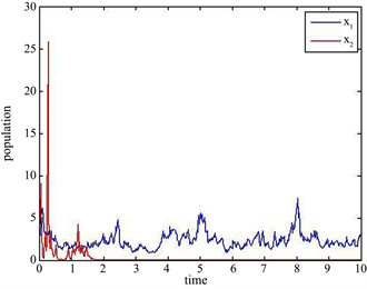
Figure 2. A solution of example 6.2 with initial value $x (0) = {(3, 5)}^{T}$

图2. 例6.2的初值为 $x (0) = {(3, 5)}^{T}$ 的解

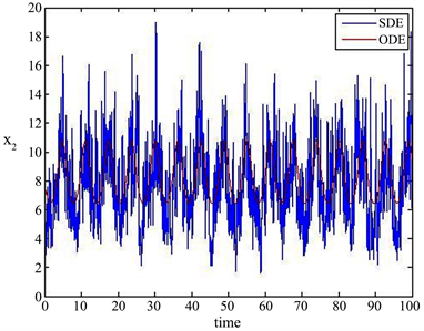
Figure 3. Solutions of example 6.3 and its determined counterpart with initial value $x (0) = {(3, 5)}^{T}$

图3. 例6.3及其对应确定性方程的初值为 $x (0) = {(3, 5)}^{T}$ 的解

基金项目

本文得到国家自然科学基金项目(11271110)和河南省教育厅科技攻关项目(15A120009)的支持。

文章引用

郭奥,丁孝全. 一类非自治随机互惠系统的渐近性态
Asymptotic Behavior of a Non-Autonomous Stochastic Mutualism System[J]. 理论数学, 2019, 09(04): 514-526. https://doi.org/10.12677/PM.2019.94068

参考文献

1. Boucher, D.H. (1985) The Biology of Mutualism: Ecology and Evolution. Oxford University Press, New York.

2. 陈凤德, 谢向东. 合作种群模型动力学研究[M]. 北京: 科学出版社, 2014.

3. Graves, W.G., Peckham, B. and Pastor, J. (2006) A Bifurcation Analysis of a Differential Equations Model for Mutualism. Bulletin of Mathematical Biology, 68, 1851-1872.
https://doi.org/10.1007/s11538-006-9070-3

4. 向红, 张小兵, 孟新友. 一类互惠模型的持续生存与周期解[J]. 兰州交通大学学报, 2009, 28(4): 156-158.

5. Gard, T.C. (1986) Stability for Multispecies Population Models in Random Environments. Nonlinear Analysis, 10, 1411-1419.
https://doi.org/10.1016/0362-546X(86)90111-2

6. Mao, X., Renshaw, E. and Marion, G. (2002) Environmental Brownian Noise Suppresses Explosions in Population Dynamics. Stochastic Processes and Their Applications, 97, 95-110.
https://doi.org/10.1016/S0304-4149(01)00126-0

7. Rudnicki, R. and Pichór, K. (2007) Influence of Stochastic Per-turbation on Prey-Predator Systems. Mathematical Biosciences, 206, 108-119.
https://doi.org/10.1016/j.mbs.2006.03.006

8. Liu, M. and Wang, K. (2011) Persistence and Extinction in Stochastic Non-Autonomous Logistic Systems. Journal of Mathematical Analysis and Applications, 375, 443-457.
https://doi.org/10.1016/j.jmaa.2010.09.058

9. Mandal, P.S. and Banerjee, M. (2012) Stochastic Persistence and Sta-tionary Distribution in a Holling-Tanner Type Prey-Predator Model. Physica A, 391, 1216-1233.
https://doi.org/10.1016/j.physa.2011.10.019

10. 王克. 随机生物数学模型[M]. 北京: 科学出版社, 2010.

11. 吕敬亮. 几类随机生物种群模型性质的研究[D]: [博士学位论文] . 哈尔滨: 哈尔滨工业大学, 2011.

12. Ji, C. and Jiang, D. (2012) Persistence and Non-Persistence of a Mutualism System with Stochastic Perturbation. Discrete and Continuous Dynamical Systems, 32, 867-889.
https://doi.org/10.3934/dcds.2012.32.867

13. Liu, M. and Wang, K. (2013) Popula-tion Dynamical Behavior of Lotka-Volterra Cooperative Systems with Random Perturbations. Discrete and Continuous Dy-namical Systems, 33, 2495-2522.
https://doi.org/10.3934/dcds.2013.33.2495

14. Liu, M. and Wang, K. (2013) Analy-sis of a Stochastic Autonomous Mutualism Model. Journal of Mathematical Analysis and Applications, 402, 392-403.
https://doi.org/10.1016/j.jmaa.2012.11.043

15. Qiu, H., Lv, J. and Wang, K. (2013) Two Types of Permanence of a Stochastic Mutualism Model. Advances in Difference Equations, 2013, 37.
https://doi.org/10.1186/1687-1847-2013-37

16. Li, M., Gao, H., Sun, C. and Gong, Y. (2015) Analysis of a Mutualism Model with Stochastic Perturbations. International Journal of Biomathematics, 8, Article ID: 1550072.
https://doi.org/10.1142/S1793524515500722

17. Guo, S. and Hu, Y. (2017) Asymptotic Behavior and Numerical Simulations of a Lotka-Volterra Mutualism System with White Noises. Advances in Difference Equations, 2017, 125.
https://doi.org/10.1186/s13662-017-1171-9

18. Gao, H. and Wang, Y. (2019) Stochastic Mutualism Model under Re-gime Switching with Lévy Jumps. Physica A, 515, 355-375.
https://doi.org/10.1016/j.physa.2018.09.189

19. Han, Q. and Jiang, D. (2015) Periodic Solution for Stochastic Non-Autonomous Multispecies Lotka-Volterra Mutualism Type Eco-system. Applied Mathematics and Computation, 262, 204-217.
https://doi.org/10.1016/j.amc.2015.04.042

20. Zhang, X., Jiang, D., Alsaedi, A. and Hayat, T. (2016) Periodic Solutions and Stationary Distribution of Mutualism Models in Ran-dom Environments. Physica A, 460, 270-282.
https://doi.org/10.1016/j.physa.2016.05.015

21. Wang, B., Gao, H. and Li, M. (2017) Analysis of a Non-Autonomous Mutualism Model Driven by Lévy Jumps. Discrete and Continuous Dy-namical Systems: Series B, 21, 1189-1202.
https://doi.org/10.3934/dcdsb.2016.21.1189

22. Karatzas, I. and Shreve, S.E. (1991) Brownian Motion and Stochastic Calculus. 2nd Edition, Springer, Berlin.

23. Mao, X. (2007) Stochastic Differential Equations and Applications. 2nd Edition, Horwood Publishing, Chichester.

24. Khasminskii, R. (2012) Stochastic Stability of Differential Equations. 2nd Edition, Springer, Berlin.
https://doi.org/10.1007/978-3-642-23280-0

25. Higham, D.J. (2001) An Algorithmic Introduction to Numerical Sim-ulation of Stochastic Differential Equations. SIAM Review, 43, 525-546.
https://doi.org/10.1137/S0036144500378302

26. Barbălat, I. (1959) Systèmes D’équations Différentielles D’oscillations Nonlinéaires. Revue Roumaine de Mathématique Pures et Appliquées, 4, 267-270.

NOTES

^*通讯作者。

期刊菜单