Dynamical Systems and Control
Vol.
08
No.
04
(
2019
), Article ID:
32404
,
8
pages
10.12677/DSC.2019.84028
Mean Square Asymptotic Stability of Stochastic Hopfield Neural Networks with Mixed Delays
Yahua Tan, Jianguo Tan
Tianjin Polytechnic University, Tianjin

Received: Sep. 10th, 2019; accepted: Sep. 22nd, 2019; published: Sep. 29th, 2019

ABSTRACT
This paper considers a stochastic Hopfield neural network model with mixed delays, the mixed delays of the model are composed of constant fixed delay and continuously distributed delay. Li and Ding (2017) introduced this model and discussed its properties. In this paper, we will continue to study this model. Therefore, the main purpose of this paper is to obtain the criteria for the mean-square asymptotic stability of stochastic Hopfield neural networks with mixed delays through research and analysis. In addition, the methods we used are Lyapunov function method, Itô’s formula method and inequality method. First of all, we construct a suitable Lyapunov function. Then we apply Itô’s formula to the Lyapunov function. By calculation, we obtain the condition for judging the mean-square asymptotic stability of stochastic Hopfield neural networks with mixed delays. Lastly, we give an example to verify the results we obtained.
Keywords:Stochastic Hopfield Neural Networks with Mixed Delays, Lyapunov Functional, Itô’s Formula, Mean Square Asymptotic Stability
混合时滞随机Hopfield神经网络的均方渐近 稳定性
谭亚华,谭建国
天津工业大学,天津
收稿日期:2019年9月10日;录用日期:2019年9月22日;发布日期:2019年9月29日

摘 要
这篇文章考虑的是具有混合时滞的随机Hopfield神经网络模型,模型的混合时滞是由常固定时滞和连续分布时滞组成。李和丁(2017)引入了这种模型并且讨论了其性质,本文将继续对这种模型进行研究。因此,文章的主要目的是通过研究、分析来获得具有混合时滞的随机Hopfield神经网络的均方渐近稳定性的判定条件。除此之外,我们使用的方法是李雅普诺夫函数法、Ito公式法和不等式法。文章首先构造了合适的李雅普诺夫函数,然后对所构造的李雅普诺夫函数应用Ito公式,通过计算从而得到了判断具有混合时滞的随机Hopfield神经网络的均方渐近稳定性的条件。最后,我们给出了一个例子来验证我们所得到的结果。
关键词 :混合时滞随机Hopfield神经网络,李雅普诺夫函数,Ito公式,均方渐进稳定性

Copyright © 2019 by author(s) and Hans Publishers Inc.
This work is licensed under the Creative Commons Attribution International License (CC BY).
http://creativecommons.org/licenses/by/4.0/


1. 引言
神经网络因其广泛的应用而受到越来越多的关注,例如,联想记忆,优化计算,信号处理,模式识别等 [1] [2] [3] [4]。此外,稳定性问题是神经网络领域中的重要问题之一,因此,许多研究者对神经网络的稳定性进行了研究,并且有一些文献可供参考 [5] [6] [7] [8] [9]。
在现实中,突触传递是由神经递质释放和其他概率原因的随机波动带来的噪声过程 [10]。因此,研究受随机因素影响的神经网络的稳定性是非常重要的。例如, [11] 研究了随机神经网络的指数稳定性和不稳定性。此外,由于时间时滞在许多神经网络模型中是不可避免的,例如,神经处理和信号传输。因此,研究随机时滞神经网络具有重要的意义。目前,关于随机时滞神经网络的研究已有一些文献。 [12] 应用变分参数、不等式技术和随机分析方法,研究了随机时滞Hopfield神经网络的均方指数稳定性。 [13] 使用Ito公式和非负半鞅收敛定理研究了随机时滞Hopfield神经网络的指数稳定性。文献 [14] 使用李雅普诺夫泛函法和线性矩阵不等式讨论了不确定随机时滞神经网络均方指数稳定性。 [15] 研究了具有分布时滞的随机递归神经网络的均方全局渐近稳定性。 [16] 通过构造李雅普诺夫函数考虑了时变离散分布时滞的随机Hopfield神经网络的均方指数稳定性。
众所周知, [17] 引入了具有混合时滞的随机Hopfield神经网络模型并且应用Ito公式和不等式技术研究了该模型的均方指数稳定性。对于具有混合时滞的随机细胞神经网络, [18] 利用李雅普诺夫函数法讨论了几乎确定的指数稳定性和p阶矩指数稳定性。然而,据我们所知,关于具有混合时滞的随机Hopfield神经网络的均方渐近稳定性的结果很少。因此,在本文中,我们的主要目的是完成这项工作。此外,通过构造合适的李雅普诺夫函数并且对该函数应用Ito公式,我们讨论了稳定性问题。
本文由以下几部分组成。在第二节中,我们介绍了文章中使用的模型、符号和假设。在第三节中我们得到了判断具有混合时滞的随机Hopfield神经网络的均方渐进稳定性的条件。在第四节中,我们给出了一个例子来验证我们的结果。最后一节,我们给出了本文的结论。
2. 模型,符号和假设
在本文中,我们考虑了由李和丁 [17] 引入的具有混合时滞的随机Hopfield神经网络模型,模型的表达式如下:
(1)
或者等价为
(2)
其中
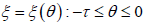
, 是网络中神经元的数量,
是在时间t第i个神经元的状态变量,
,,, 和
是在时间t和
第j个神经元的激活函数,
 是正定对角矩阵,
, 和
分别是反馈矩阵和时滞反馈矩阵,核
,, 和
是连续函数,
是传输时滞,
。接下来,我们介绍了本文使用的下列符号。
是正定对角矩阵,
, 和
分别是反馈矩阵和时滞反馈矩阵,核
,, 和
是连续函数,
是传输时滞,
。接下来,我们介绍了本文使用的下列符号。
设 是一个具有滤子
且满足通常条件的完全概率空间,即,当
包含所有P-空集时,它是右连续的和递增的。
是从
到
的连续函数族,其范数为
并且
。
定义了一族所有
可测有界
值随机变量
是一个具有滤子
且满足通常条件的完全概率空间,即,当
包含所有P-空集时,它是右连续的和递增的。
是从
到
的连续函数族,其范数为
并且
。
定义了一族所有
可测有界
值随机变量
 。
是n维布朗运动。对于
, 和
互相独立,E是期望。
。
是n维布朗运动。对于
, 和
互相独立,E是期望。
设 定义了一族 上对x二次可微,对t一次可微的非负函数 。定义
系统(1)的算子 如下:
(3)
其中
,
 ,
,
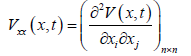 ,
。
,
。
2.1. 假设
a) 函数 ,,, 和 满足:
,且 ,。
b) 函数 ,, 和 是利普希茨连续的,即,存在非负常数 ,,, 使得
(4)
(5)
(6)
(7)
c) 下面的不等式是成立的:
 (8)
(8)
如果存在矩阵 ,,,。
2.2. 定义
对于每个初值 ,如果 ,则系统(1)的平衡点是均方渐近稳定的。
3. 主要的结果
定理:在假设a)~c)下,系统(1)的零平衡点是均方渐近稳定的,如果存在矩阵 使得
其中 ,,,。
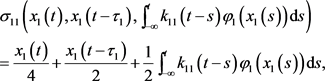
证明:下面是我们构建的李雅普诺夫函数。
对于系统(1),我们应用Ito公式并且估计 如下:
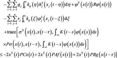
(9)
根据不等式 ,我们有
(10)
(11)
(12)
通过(9)~(12),我们得到
因此,我们得到 。即,系统(1)的零平衡点是均方渐近稳定的。
4. 例子
考虑具有混合时滞的二维随机Hopfield神经网络。
(13)
取C,A,B和D如下:
设 ,,,,然后我们有 ,,,。
选择 ,,,这样我们有
因此,根据定理的内容,我们得到神经网络是均方渐近稳定的。
5. 结论
本文考虑的是具有混合时滞的随机Hopfield神经网络模型,本文首先构造了合适的李雅普诺夫函数,然后对所构造的李雅普诺夫函数应用Ito公式,通过进一步的计算得到了具有混合时滞的随机Hopfield神经网络的均方渐近稳定性的判定条件。最后,我们给出了一个例子验证了所得到的结果。
基金项目
天津自然科学基金会(No: 17JCQNJC03800)。
文章引用
谭亚华,谭建国. 混合时滞随机Hopfield神经网络的均方渐近稳定性
Mean Square Asymptotic Stability of Stochastic Hopfield Neural Networks with Mixed Delays[J]. 动力系统与控制, 2019, 08(04): 263-270. https://doi.org/10.12677/DSC.2019.84028
参考文献
- 1. Hopfield, J. (1982) Neural Networks and Physical Systems with Emergent Collective Computational Abilities. Proceedings of the National Academy of Sciences, 79, 2554-2558.
https://doi.org/10.1073/pnas.79.8.2554 - 2. 郭鹏, 韩璞. Hopfield网络在优化计算中的应用[J]. 计算机仿真, 2002, 19(3): 37-39.
- 3. 韩琦. 神经网络的稳定性及其在联想记忆中的应用研究[D]: [博士学位论文]. 重庆: 重庆大学计算机学院, 2012.
- 4. Shitonga, W., Duana, F., Mina, X. and Dewenc, H. (2007) Advanced Fuzzy Cellular Neural Networks: Application to CT Liver Images. Artificial Intelligence in Medicine, 39, 65-77.
https://doi.org/10.1016/j.artmed.2006.08.001 - 5. Arik, S. (2000) Global Asymptotic Stability of a Class of Dynamical Neural Networks. IEEE Transactions on Circuits and Systems—I: Fundamental Theory and Applications, 47, 568-571.
https://doi.org/10.1109/81.841858 - 6. 徐晓惠, 张继业, 施继忠, 等. 脉冲干扰时滞复值神经网络的稳定性分析[J]. 哈尔滨工业大学学报, 2016, 48(3): 166-170.
- 7. Bai, J., Lu, R., Xue, A., et al. (2015) Finite-Time Stability Analysis of Discrete-Time Fuzzy Hopfield Neural Network. Neurocomputing, 159, 263-267.
https://doi.org/10.1016/j.neucom.2015.01.051 - 8. Xu, B., Liu, X. and Liao, X. (2006) Global Exponential Stability of High Order Hopfield Type Neural Networks. Applied Mathematics and Computation, 174, 98-116.
https://doi.org/10.1016/j.amc.2005.03.020 - 9. Zhu, Q. and Cao, J. (2014) Mean-Square Exponential Input-to-state Stability of Stochastic Delayed Neural Networks. Neurocomputing, 131, 157-163.
https://doi.org/10.1016/j.neucom.2013.10.029 - 10. Haykin, S. (1994) Neural Netw. Prentice-Hall, Upper Saddle Riv-er.
- 11. Liao, X. and Mao, X. (1996) Exponential Stability and Instability of Stochastic Neural Networks. Stochastic Analysis and Applications, 14, 165-185.
https://doi.org/10.1080/07362999608809432 - 12. Wan, L. and Sun, J. (2005) Mean Square Expo-nential Stability of Stochastic Delayed Hopfield Neural Networks. Physics Letters A, 343, 306-318.
https://doi.org/10.1016/j.physleta.2005.06.024 - 13. Zhou, Q. and Wan, L. (2008) Exponential Stability of Stochastic Delayed Hopfield Neural Networks. Applied Mathematics and Computation, 199, 84-89.
https://doi.org/10.1016/j.amc.2007.09.025 - 14. Chen, W. and Lu, X. (2013) Mean Square Exponential Stability of Uncertain Stochastic Delayed Neural Networks. Physics Letters A, 372, 1061-1069.
https://doi.org/10.1016/j.physleta.2007.09.009 - 15. Guo, Y. (2009) Mean Square Global Asymptotic Stability of Stochastic Recurrent Neural Networks with Distributed Delays. Applied Mathematics and Computation, 215, 791-795.
https://doi.org/10.1016/j.amc.2009.06.002 - 16. Ma, L. and Da, F. (2009) Mean-Square Exponential Stability of Stochastic Hopfield Neural Networks with Time-Varying Discrete and Distributed Delays. Physics Letters A, 373, 2154-2161.
https://doi.org/10.1016/j.physleta.2009.04.031 - 17. Li, X. and Deng, D. (2017) Mean Square Exponential Stability of Stochastic Hopfield Neural Networks with Mixed Delays. Statistics & Probability Letters, 126, 88-96.
https://doi.org/10.1016/j.spl.2017.02.029 - 18. Li, X., Deng, D. and Di, S. (2018) Exponential Stability of Stochastic Cellular Neural Networks with Mixed Delays. Communications in Statistics—Theory and Methods, 47, 4881-4894.