Statistics and Application
Vol.
10
No.
02
(
2021
), Article ID:
41711
,
15
pages
10.12677/SA.2021.102024
基于时间序列模型对澳元兑美元汇率的研究
张钰
曲阜师范大学统计学院,山东 曲阜

收稿日期:2021年3月25日;录用日期:2021年4月9日;发布日期:2021年4月21日

摘要
汇率是国际贸易中的调节杠杆,对进出口贸易收支、国内物价水平、国际资本流动和经济结构、生产布局等都会产生重要影响,因此研究汇率变动有十分重要的意义。本文主要研究澳元兑美元的汇率数值变动,选取澳元兑美元汇率变动较为显著的1979~1999年的数据进行时间序列分析,本文分别对数据拟合了ARIMA模型和GARCH模型,对模型进行各项检验,并比较了两种模型的优劣,且与目前已获得的在此之后的真实汇率值作比较以评估模型的拟合效果,最终选择GARCH模型来拟合澳元兑美元的汇率变动,并在此结果的基础上说明GARCH模型在金融数据中的广泛应用。
关键词
澳元兑美元汇率变动,ARIMA模型,GARCH模型,时间序列分析
Study on the Exchange Rate of Australian Dollar against US Dollar Based on Time Series Model
Yu Zhang
School of Statistics, Qufu Normal University, Qufu Shandong

Received: Mar. 25th, 2021; accepted: Apr. 9th, 2021; published: Apr. 21st, 2021

ABSTRACT
Exchange rate is a regulatory lever in international trade. It has an important impact on import and export trade balance, domestic price level, international capital flow and economic structure and production layout. Therefore, it is of great significance to study exchange rate fluctuations. This paper mainly studies the numerical changes of the exchange rate of Australian dollar against the US dollar, and selects the data from 1979 to 1999 when the exchange rate of Australian dollar against the US dollar changed significantly for time series analysis. In this paper, ARIMA model and GARCH model are fitted to the data respectively, various tests are carried out on the models, and the advantages and disadvantages of the two models are compared, and the real exchange rate values obtained after this are compared to evaluate the fitting effect of the models. Finally, the GARCH model is chosen to fit the exchange rate change of Australian dollar against US dollar, and the extensive application of GARCH model in financial data is illustrated on the basis of the results.
Keywords:Australian Dollar/US Dollar Exchange Rate, ARIMA Model, GARCH Model, Time Series Analysis

Copyright © 2021 by author(s) and Hans Publishers Inc.
This work is licensed under the Creative Commons Attribution International License (CC BY 4.0).
http://creativecommons.org/licenses/by/4.0/


1. 引言
汇率变动一直是各个国家向来关注的热点问题,汇率变动对一国国内就业、国民收入及资源配置乃至世界经济都有重要的影响。本文在查阅资料后,发现澳元兑美元汇率在上个世纪末有明显的变动,因此选择这一时间段进行研究。利用时间序列模型和R软件对数据进行分析,希望获得一个较好的澳元兑美元汇率走势的拟合模型。
2. 材料与方法
2.1. 研究背景
汇率是两种货币之间兑换的比率,汇率变动对一个国家的进出口贸易有着直接的调节作用 [1]。通过查阅资料,了解到20世纪70年代到20世纪90年代末澳元兑美元的汇率有明显的变动。本文在获取该时间段的澳元兑美元汇率数据后(数据来源见附录),选取适当的模型,旨在对其走势进行拟合,并且比较两种模型的优劣。
2.2. 澳元兑美元汇率的研究模型
本文依托选取的数据,分别对数据采用ARIMA模型和GARCH模型进行拟合,旨在比较两种模型的优缺点,并判断模型拟合效果的优劣。
2.2.1. 求和自回归移动平均(ARIMA)模型
具有如下结构的模型称为求和自回归移动平均模型,简记为ARIMA (p, d, q)模型:
可以看到,使用ARIMA模型需满足以下三个条件:
条件一:随机干扰序列 为零均值白噪声序列。
条件二:当期的随机干扰与过去的序列值无关。
条件三:残差序列方差齐性。
2.2.2. 广义自回归条件异方差(GARCH)模型
一个完整的GARCH (p, q)模型的结构如下:
参数满足如下约束条件:
该模型包括均值模型、条件异方差模型和分布假定。GARCH模型打破了传统的方差恒定的假设,该模型的提出解决了许多之前未曾解决的问题。
3. 结果与分析
3.1. ARIMA模型的建立
绘制时序图是对时间序列数据进行分析的第一步。该序列的时序图如图1所示。

Figure 1. Timing chart of the Australian dollar against the US dollar
图1. 澳元兑美元汇率时序图
观察时序图可知,该序列有显著的趋势,为典型的非平稳序列。下面对该序列进行一阶差分,以提取序列的确定性趋势信息。差分后的时序图如图2所示。
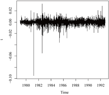
Figure 2. Time sequence chart of Australian dollar against US dollar after 1st order difference
图2. 澳元兑美元汇率1阶差分后序列时序图
差分后序列已经没有非常明显的趋势特征,为进一步确定差分后序列的平稳性,下面对差分后的序列进行平稳白噪声(ADF)检验,检验结果见表1。

Table 1. First order difference sequence ADF test results
表1. 一阶差分序列ADF检验结果
检验结果显示,该序列所有统计量的P值均小于给定的显著性水平 ,所以可以认定一阶差分后的序列实现了平稳。下面对一阶差分后的序列进行纯随机性检验,检验结果如表2所示。
Table 2. Test results of pure randomness of first order difference sequences
表2. 一阶差分序列纯随机性检验结果
检验结果显示,各阶延迟下LB统计量的P值都小于给定的显著性水平 ,所以认为一阶差分后的序列为平稳非白噪声序列。下面对一阶差分后序列拟合ARMA模型,图3和图4为一阶差分序列的自相关系数图和偏自相关系数图。
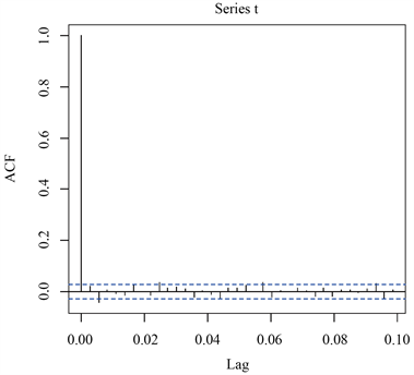
Figure 3. Autocorrelation coefficient diagram of first-order difference sequence
图3. 一阶差分序列自相关系数图

Figure 4. Partial autocorrelation coefficient diagram of first- order difference series
图4. 一阶差分序列偏自相关系数图
根据图3和图4所表现出的特征,可以认为一阶差分后序列的自相关系数和偏自相关系数均表现出拖尾的性质,因此,对差分后的序列尝试拟合ARMA (1, 1)模型,即对原序列尝试拟合ARIMA (1, 1, 1)模型,运行结果如表3。
Table 3. ARIMA(1,1,1) model parameter estimation
表3. ARIMA(1,1,1)模型参数估计
根据公式 ,计算可得如下模型结构:
,
对ARIMA模型的拟合结果进行残差白噪声检验和参数显著性检验,检验结果见表4。
Table 4. Checklist of fitting results
表4. 拟合结果检验表
根据以上检验结果可知,模型通过了检验,可以用来进行下一步的预测。预测未来10日的汇率数值,结果如下:
0.6635970 0.6636576 0.6636220 0.6636429 0.6636306 0.6636378 0.6636336
0.6636361 0.6636346 0.6636355
查阅当时的真实汇率数据,发现该模型的拟合结果与真实数据基本吻合,预测效果较好。
3.2. GARCH模型的建立
集群效应是经济和金融领域常见的现象 [2]。集群效应的存在意味着方差非齐,此时就不符合ARIMA模型中方差齐性的假设,导致得到的置信区间达不到要求。根据一阶差分后的序列的时序图,可以看出存在集群效应,下面对该数据拟合GARCH模型 [3]。
首先对一阶差分后的序列进行PP检验,检验结果如下(表5):
Table 5. PP test results
表5. PP检验结果
P值等于0.01,这说明差分后序列可视为平稳序列,接下来对差分后序列进行纯随机性检验,检验结果同表2,同时考察差分后序列的自相关系数大小,结果如下(表6):
Table 6. Autocorrelation coefficients of each order of delay
表6. 延迟各阶的自相关系数
LB检验的P值都极小,所以白噪声检验结果是该序列为非白噪声序列,但延迟各阶的自相关系数显示序列值之间的相关性很小,综合考虑,可以认为差分后序列近似为纯随机序列。至此,认为汇率的均值模型为ARIMA (0, 1, 0)模型,即随机游走模型:
下面对差分后的序列进行条件异方差检验(表7)。
Table 7. Conditional heteroscedasticity test results
表7. 条件异方差检验结果
Q检验和LM检验均显著拒绝方差齐性假定,可以认为残差平方序列中蕴含显著的相关信息,值得拟合条件异方差模型进行提取。
下面拟合GARCH (1, 1)模型,运行结果如下(表8):
Table 8. Parameter estimation of GARCH (1, 1) model and significance test results
表8. GARCH (1, 1)模型参数估计值及显著性检验结果
由表8可以发现omega没有通过显著性检验,可以剔除。模型输出的信息量为:
Information Criteria
------------------------------------
Akaike −8.0918
Bayes −8.0879
Shibata −8.0918
Hannan-Quinn −8.0905
至此,基于条件最小二乘估计方法,得到的拟合模型如下:
GARCH模型通常认为序列服从正态分布,但在某些情况下序列未必服从正态分布,下面对这个分布假定进行检验。画出模型残差序列的QQ图和直方图如图5和图6。
从QQ图可以看到残差序列的真实分位点偏离正态参考线,且残差直方图显示序列观察值比标准正态分布高耸,这说明序列并不服从正态分布假定。下面尝试将正态分布改为t分布,结果如表9。
模型输出的信息量为:
Information Criteria
------------------------------------
Akaike −8.3075
Bayes −8.3023
Shibata −8.3075
Hannan-Quinn −8.3057

Figure 5. QQ chart of model residuals
图5. 模型残差QQ图
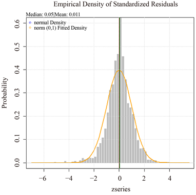
Figure 6. Histogram of model residuals
图6. 模型残差直方图
Table 9. The GARCH(1,1) parameter estimation and significance test results after changing to t distribution
表9. 改为t分布后GARCH(1,1)参数估计值及显著性检验结果
此时可以发现,模型的AIC和BIC信息量都比之前要小,拟合效果较之前略优,拟合模型为:
以上两种模型的显著性检验分别如下(表10~13):
Table 10. White noise test results of standardized residual sequence
表10. 标准化残差序列的白噪声检验结果
Table 11. White noise test results of standardized residual-squared sequences
表11. 标准化残差平方序列的白噪声检验结果
Table 12. The white noise test results of standardized residual sequence after t distribution is changed
表12. 改为t分布后标准化残差序列的白噪声检验结果
Table 13. The white noise test results of standardized residual-square sequence after t distribution
表13. 改为t分布后标准化残差平方序列的白噪声检验结果
通过检验可以发现,在显著性水平 下拟合的均值模型并未通过显著性检验,是选择的均值模型没能充分地提取序列中蕴含的水平信息,但对波动信息的提取非常充分,下面尝试对均值模型进行改进,我们仍改用ARIMA (1, 1, 1)模型提取水平信息,得到最终模型:
均值模型的结构已在ARIMA建模时说明。下面对模型进行检验,由表14和表15可知此时模型通过了显著性检验。
Table 14. The white noise test results of the standardized residual sequence after the improved mean model were obtained
表14. 改进均值模型后标准化残差序列白噪声检验结果
Table 15. Standardized white noise test results of residual-square sequence after improved mean model
表15. 改进均值模型后标准化残差平方序列白噪声检验结果
图7给出的是分别在方差齐性假定下得到的95%的置信区间和最终拟合的GARCH (1, 1)模型拟合的条件异方差得到的95%的置信区间,当序列大幅波动时,条件异方差模型的置信区间大于方差齐性置信区间;而在序列小值波动时,条件异方差模型的置信区间小于方差齐性置信区间,更接近序列的真实波动情况,对序列的预测更加准确,更能提供有用可信的信息。

Figure 7. Schematic comparison of conditional and unconditional heteroscedasticity
图7. 条件异方差和无条件异方差的比较示意图
使用该模型预测未来10日的汇率数据,结果如下(表16):
Table 16. 95% confidence interval for the next 10 issues
表16. 未来10期95%置信区间
4. 总结
本文基于获得的澳元兑美元汇率数据,利用时间序列的分析方法,借助R软件,先后采用ARIMA模型和GARCH模型对数据进行拟合,并比较了两个模型的优劣,并与获得的真实数据与预测数据进行比较。最终确定GARCH模型能较好地拟合澳元兑美元汇率趋势变动。GARCH模型在金融领域的应用更为广泛。随着科学技术的发展,人们对GARCH模型不断改良,衍生出许多更加优化的模型对数据进行分析和预测。
文章引用
张 钰. 基于时间序列模型对澳元兑美元汇率的研究
Study on the Exchange Rate of Australian Dollar against US Dollar Based on Time Series Model[J]. 统计学与应用, 2021, 10(02): 241-255. https://doi.org/10.12677/SA.2021.102024
参考文献
- 1. 马思涛. 基于时间序列模型对人民币汇率的研究[J]. 知识经济, 2019(33): 43-45.
- 2. 李明轩, 俞翰君. 基于ARMA-GARCH模型的人民币汇率波动性研究[J]. 时代金融, 2020(33): 1-3+8.
- 3. 王倩倩, 卫龙宝, 王文亭. 基于GARCH类模型中国原料奶价格波动实证分析[J]. 农业经济问题, 2020(11): 97-107.
附录
澳元兑美元汇率数据
本文所研究的澳元兑美元汇率数据来自网站:
https://cn.investing.com/currencies/aud-usd-historical-data
时间序列分析R代码
#拟合ARMA模型
setwd(E://R语言学习)
data=read.csv(AUD_USD历史数据.csv,header=TRUE)
data
x=data$收盘
x
x1=ts(x,frequency=365,start=c(1979,12,27))
plot(x1)
windows()
t=diff(x1)
plot(t)
install.packages(aTSA)
library(aTSA)
acf(t)
pacf(t)
adf.test(t)
install.packages(forecast)
library(forecast)
predict(arima(x,order=c(1,1,1)),n.ahead=10)#预测未来10天的汇率值
x.fore=predict(arima(x,order=c(1,1,1)),n.ahead=10)
U=x.fore$pred+1.96*x.fore$se
L=x.fore$pred-1.96*x.fore$se
x.fit<-arima(x,order=c(1,1,1),method=CSS)
x.fit
ev=x.fit$residuals
ev
for(i in 1:3) print(Box.test(ev,type=Ljung-Box,lag=6*i))
t1=-0.5882/0.1725
t2=0.6197/0.1663#参数显著性检验
p1=pt(t1,df=4994,lower.tail=TRUE)*2
p2=pt(t2,df=4994,lower.tail=FALSE)*2
p1
p2
#拟合GARCH模型
PP.test(t)
for(i in 1:3) print(Box.test(t,lag=6*i,type=Ljung-Box))
print(acf(diff(x),lag=24))
spec1<-ugarchspec(
mean.model=list(armaOrder=c(0,0),include.mean=FALSE),
variance.model=list(garchOrder=c(1,1),model=sGARCH),
distribution.model=norm)
fit1<-ugarchfit(spec1,data=t)
fit1
plot(fit1,which=8)
plot(fit1,which=9)
spec2<-ugarchspec(
mean.model=list(armaOrder=c(0,0),include.mean=FALSE),
variance.model=list(garchOrder=c(1,1),model=sGARCH),
distribution.model=std)
fit2<-ugarchfit(spec1,data=t)
fit2
x.fit<-arima(x,order=c(1,1,1))
arch.test(x.fit)
install.packages(rugarch)
library(rugarch)
spec3<-ugarchspec(
mean.model=list(armaOrder=c(1,1),include.mean=FALSE),
variance.model=list(garchOrder=c(1,1),model=sGARCH),
distribution.model=norm)
fit3<-ugarchfit(spec1,data=t,method=CLS)
fit3
plot(fit3,which=1)
abline(h=c(-1.96*sd(diff(x)),1.96*sd(diff(x))),col=1,lwd=2,lty=2)
a=(fit3@fit$sigma[length(fit3@fit$sigma)])^2
a
ht=0
for(i in 1:5){
ht[i]=fit3@fit$coef[1]+(fit3@fit$coef[2]+fit3@fit$coef[3])*a
a=ht[i]
}
sumh<-cumsum(ht)
xt<-x[length(x)]
sigma<-sqrt(ht)
sigma_fore<-sqrt(sumh)
L=xt-1.96*sigma_fore
U=xt+1.96*sigma_fore
data.frame(xt,sigma_fore,L,U)