Advances in Applied Mathematics
Vol.
08
No.
02
(
2019
), Article ID:
28843
,
8
pages
10.12677/AAM.2019.82025
The Exact Solutions of the Sharma-Tasso-Olver Equation Using exp(-G(ξ)) Method and Ansatz Method
Fengyan Zhang1,2, Dongxue Li3, Junmei Wang1
1School of Mathematics and Statistics, Shandong Normal University, Jinan Shandong
2School of Mathematics and Statistics, Shandong Linyi University, Linyi Shandong
3Dezhou No. 10 Middle School, Dezhou Shandong

Received: Jan. 22nd, 2019; accepted: Feb. 6th, 2019; published: Feb. 13th, 2019

ABSTRACT
Using the traveling wave transformation and homogeneous balance simplified the Sharma-Tasso-Olver equation to obtain the reduced ordinary differential equations, using the -method to get the trigonometric function solution, hyperbolic function solution and the rational function solution. In addition, an exact soliton solution is provided by using the Ansatz method.
Keywords:Sharma-Tasso-Olver Equation, -Method, Soliton Solution, Ansatz Method

利用exp(-G(ξ))方法和拟设函数法求Sharma-Tasso-Olver方程精确解
张逢燕1,2,李冬雪3,王俊梅1
1山东师范大学,数学与统计学院,山东 济南
2临沂大学,数学与统计学院,山东 临沂
3德州市第十中学,山东 德州

收稿日期:2019年1月22日;录用日期:2019年2月6日;发布日期:2019年2月13日

摘 要
本文运用行波变换和齐次平衡原理对Sharma-Tasso-Olver方程进行化简,得到约化的常微分方程。利用 方法和拟设双曲函数法求得方程的三角函数解、双曲函数解、有理函数解和孤子解。
关键词 :Sharma-Tasso-Olver方程, 方法,孤子解,拟设双曲函数法

Copyright © 2019 by authors and Hans Publishers Inc.
This work is licensed under the Creative Commons Attribution International License (CC BY).
http://creativecommons.org/licenses/by/4.0/


1. 引言
非线性发展方程是国内外研究的热点问题,Sharma-Tasso-Olver (STO)方程在数学和物理领域有着重要的作用,很多专家对其有深入研究。例如,文献 [1] [2] 运用Bäcklund变换求精确解。在 [3] 中介绍扩展双曲函数方法的STO方程的显式行波解。楼森岳等人 [4] 通过使用标准的截断Painlevé分析,Hirota双线性方法和Bäcklund变换方法彻底检查了孤子裂变和聚变。在 [5] 中,Yan通过使用两种类型的Cole-Hopf变换,研究了两类(2 + 1)维广义Sharma-Tasso-Olver积分-微分方程的可积性。他证明了这两个GSTO方程都拥有Painlevé属性和双哈密顿结构。另外,利用耦合Riccati方程方法 [6] ,修正最简单方程方法 [7] ,Exp函数方法 [8] [9] 和李对称分析求出STO方程精确解等 [10] [11] [12] 。
我们研究以下STO方程
(1)
其中 , 是任意常数。
本文首先对Sharma-Tasso-Olver方程进行了综述。第二部分运用行波变换,利用 方法 [13] [14] [15] 和齐次平衡原理 [16] [17] 将原方程约化成常微分方程,求出方程的三角函数解,双曲函数解和有理函数解。第三部分利用拟设双曲函数的行波变换得到方程的孤子解 [18] [19] 。
2. 方法
对于方程(1),我们进行行波变换:
, ,
得到约化的常微分方程:
积分一次为:
(2)
我们假设方程(2)有以下形式的精确解 [14] [15] [16] :
(3)
其中 为任意常数,m为正整数, 满足以下辅助常微分方程:
(4)
从辅助方程(4)中我们可以得到不同的精确解。
把(3)和(4)带入(2),利用齐次平衡原理可以得到 ,则方程(1)的解可以表示为:
(5)
把(4)和(5)带入(2),收集 , 的系数,令其系数方程等于0,可以得到关于 的超定方程组:
(6)
(7)
(8)
(9)
求解(6)~(9),得到两组解分别为:
情况1: ,带入方程(5),得到五种不同的解为:
① 当 ,且 时,
;(如图1)
② 当 ,且 时,
;(如图2)
③ 当 ,且 时,
;(如图3)
④ 当 ,且 时,
;(如图4)
⑤ 当 ,且 时,
,(如图5)
其中 , 为任意常数。
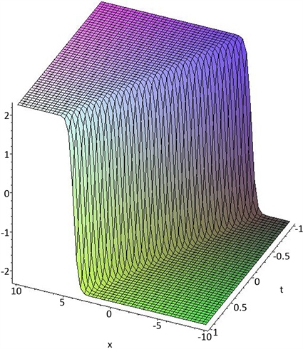
Figure 1. Hyperbolic function solution
图1. 双曲函数解
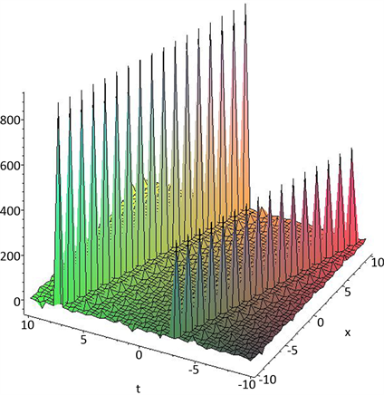
Figure 2. Trigonometric function solution
图2. 三角函数解
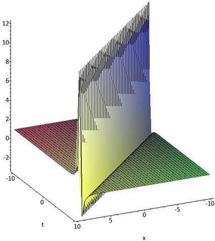
Figure 3. Hyperbolic function solution
图3. 双曲函数解
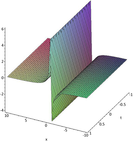
Figure 4. Rational function solution
图4. 有理函数解
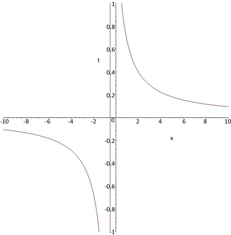
Figure 5. Rational function solution
图5. 有理函数解
情况2: ,带入方程(7),得到五种不同的解为:
① 当 ,且 时,
;
② 当 ,且 时,
;
③ 当 ,且 时,
;
④ 当 ,且 时,
;
⑤ 当 ,且 时,
,
其中 , 为任意常数。
3. 拟设双曲函数法
假设方程有以下形式的解 [18] [19] :
, , (10)
其中A和B是自由参数,p是固定参数,v是孤子速度。
由(10)可以得到:
(11)
(12)
(13)
(14)
把(11)~(14)带入方程(1),得到:
(15)
从(15)的指数可以得到 和 相等,得到 。代入(29)收集 的系数,令其系数方程等于0,可以得到:
或者 ,
上式给出了自由参数A和B的关系,扰动孤子的速度v。我们就得到了方程(1)的1-孤子解:
。
4. 结论
本文运用行波变换、齐次平衡原理,利用 方法求出Sharma-Tasso-Olver方程的新显式行波解。这些解包括双曲函数解,三角函数解和有理数解。利用拟设双曲函数得到了方程的1-孤子解。
文章引用
张逢燕,李冬雪,王俊梅. 利用exp(-G(ξ))方法和拟设函数法求Sharma-Tasso-Olver方程精确解
The Exact Solutions of the Sharma-Tasso-Olver Equation Using exp(-G(ξ)) Method and Ansatz Method[J]. 应用数学进展, 2019, 08(02): 219-226. https://doi.org/10.12677/AAM.2019.82025
参考文献
- 1. Shang, Y.D., Huang, Y. and Yuan, W.J. (2011) Bäcklund Transformations and Abundant Exact Explicit Solutions of the Sharma-Tasso-Olver Equation. Applied Mathematics and Computation, 217, 7172-7183. https://doi.org/10.1016/j.amc.2011.01.115
- 2. Fan, E.G. and Zhang, H.Q. (1998) A New Approach to Bäcklund Transformations of Nonlinear Evolution Equations. Applied Mathematics and Mechanics, 19, 645-650.
- 3. Shang, Y. (2008) The Extended Hyperbolic Functions Method and Exact Solutions to the Long-Short Wave Resonance Equations. Chaos, Solitons & Fractals, 36, 762-771. https://doi.org/10.1016/j.chaos.2006.07.007
- 4. Wang, S., Tang, X.Y. and Lou, S.Y. (2004) Soliton Fission and Fusion: Burgers Equation and Sharma-Tasso-Olver Equation. Chaos, Solitons & Fractals, 21, 231-239. https://doi.org/10.1016/j.chaos.2003.10.014
- 5. Yan, Z.Y. (2003) Integrability of Two Types of the (2 + 1)-Dimensional Generalized Sharma-Tasso-Olver Integro-Differential Equations. Acta Mathematica Scientia, 22, 302-324.
- 6. Shang, Y.D., Qin, J.H. and Huang, Y. (2008) Abundant Exact and Explicit Solitary Wave and Periodic Wave Solutions to the Sharma-Tasso-Olver Equation. Applied Mathematics and Computation, 202, 532-538. https://doi.org/10.1016/j.amc.2008.02.034
- 7. Kudryashov, N.A. and Loguinova, N.B. (2008) Extended Simplest Equation Method for Nonlinear Differential Equations. Applied Mathematics and Computation, 205, 396-402.
- 8. Bekir, A. and Boz, A. (2008) Exact Solutions for Nonlinear Evolution Equations Using Exp-Function Method. Physics Letters A, 372, 1619-1625. https://doi.org/10.1016/j.physleta.2007.10.018
- 9. Erbas, B. and Yusufoglu, E. (2009) Exp-Function Method for Constructing Exact Solutions of Sharma-Tasso-Olver Equation. Chaos, Solitons & Fractals, 41, 2326-2330. https://doi.org/10.1016/j.chaos.2008.09.003
- 10. Lian, Z.J. and Lou, S.Y. (2005) Symmetries and Exact Solutions of the Sharma-Tasso-Olver Equation. Nonlinear Anal, 63, e1167-e1177.
- 11. Inan, I.E. and Kaya, D. (2007) Exact Solutions of Some Nonlinear Partial Differential Equations. Physica A, 381, 104-115. https://doi.org/10.1016/j.physa.2007.04.011
- 12. Wazwaz, A.M. (2007) New Solitons and Kinks Solutions to the Sharma-Tasso-Olver Equation. Applied Mathematics and Computation, 188, 1205-1213. https://doi.org/10.1016/j.amc.2006.10.075
- 13. Akbulut, A., Kaplan, M. and Tascan, F. (2017) The Investigation of Exact Solutions of Nonlinear Partial Differential Equations by Using Method. Optik, 132, 382-387. https://doi.org/10.1016/j.ijleo.2016.12.050
- 14. Roshid, H.O., Alam, M.N. and Akbar, M.A. (2015) Exact Trav-eling Wave Solutions to the (3+1)-Dimensional mKdV –ZK and the (2+1)-Dimensional Burgers Equations via -Expansion Method. Alexandria Engineering Journal, 54, 635-644. https://doi.org/10.1016/j.aej.2015.05.005
- 15. Bhrawy, A.H. and Obaid, M. (2012) New Exact Solutions for the Zhiber-Shabat Equation Using the Extended F-Expansion Method. Life Sciences, 9, 1154-1162.
- 16. Fan, E.G. (2000) Two New Applications of the Homogeneous Balance Method. Physics Letters A, 265, 353-357. https://doi.org/10.1016/S0375-9601(00)00010-4
- 17. Zhang, H.Q. (2001) Extension and Application of Homogenous Balance Method. Applied Mathematics and Mechanics, 21, 321-325.
- 18. Jawad, A.J.M., Petkovic, M.D. and Biswas, A. (2010) Soliton Solutions of Burgers Equations and Perturbed Burgers Equation. Applied Mathematics and Computation, 216, 3370-3377. https://doi.org/10.1016/j.amc.2010.04.066
- 19. Wang, G.W. and Kara, A.H. (2018) Group Analysis, Fractional Explicit Solutions and Conservation Laws of Time Fractional Generalized Burgers Equation. Communications in Theoretical Physics, 69, 5-8.