Advances in Applied Mathematics
Vol.
11
No.
04
(
2022
), Article ID:
50879
,
12
pages
10.12677/AAM.2022.114236
分数阶守恒Swift-Hohenberg方程的 三种显隐Runge-Kutta方法
李婷,陈筱彦,白怡敏,胡小兵*
华侨大学数学科学学院,福建 泉州
收稿日期:2022年3月26日;录用日期:2022年4月21日;发布日期:2022年4月28日

摘要
分数阶守恒Swift-Hohenberg (SH)方程是材料学中模拟凝固微观组织的基本模型。由于分数阶导算子及非局部守恒项的影响,许多求解经典整数阶SH方程行之有效的数值方法在解决此类问题时存在严重困难。本文针对分数阶守恒SH方程,研究其高效数值逼近算法。首先,在时间方向采用显隐Runge-Kutta方法,空间方向采用傅里叶谱方法,构造分数阶守恒SH方程的数值格式;其次,进一步给出所建立格式质量守恒的理论分析;最后,通过数值实验验证了格式的收敛阶和能量递减性,同时对长时间动力行为进行模拟,验证了算法的有效性。
关键词
分数阶守恒SH方程,非局部Lagrange乘子,傅里叶谱方法,显隐Runge-Kutta方法,质量守恒

Three Explicit and Implicit Runge-Kutta Methods for Fractional Conservation Swift-Hohenberg Equation
Ting Li, Xiaoyan Chen, Yimin Bai, Xiaobing Hu*
School of Mathematical Sciences, Huaqiao University, Quanzhou Fujian
Received: Mar. 26th, 2022; accepted: Apr. 21st, 2022; published: Apr. 28th, 2022

ABSTRACT
Fractional conservation Swift-Hohenberg (SH) equation is a basic model for simulating solidification microstructure in material science. Due to the influence of fractional derivative operators and nonlocal conservation terms, many effective numerical methods for solving classical integer order SH equations have severe difficulties in solving such problems. In this paper, an efficient numerical approximation algorithm for fractional conservative SH equation is studied. Firstly, the explicit and implicit Runge-Kutta method is used in the time direction and Fourier spectrum method is used in the space direction to construct the numerical schemes of fractional order conserved SH equation. Secondly, the theoretical analysis of mass conservation of these schemes is given. Finally, the convergence order and energy decrease of these schemes are verified by numerical experiments, and the validity of these algorithms are verified by long-term dynamic behavior simulation.
Keywords:Fractional Conservation Swift-Hohenberg Equation, Nonlocal Lagrange Multiplier, Fourier Spectral Method, Implicit-Explicit Runge-Kutta Method, Mass Conservation

Copyright © 2022 by author(s) and Hans Publishers Inc.
This work is licensed under the Creative Commons Attribution International License (CC BY 4.0).
http://creativecommons.org/licenses/by/4.0/


1. 引言
相场晶体模型,是一种能够有效模拟凝固微观组织的新方法 [1],可用于模拟裂纹萌生、相分离、外延生产机制、晶界迁移和位错运动等,因此相场晶体模型成为科研学者进行微观组织研究的重要工具 [2],而Swift-Hohenberg (SH)方程就是一种重要的相场晶体模型。SH方程是由Swift和Hohenberg [3] 在1976年研究卷波的Rayleigh-Bénard不稳定性的简单模型时提出的,随后有大量学者对SH方程进行了数值求解 [4] [5] [6]。
经典的SH模型是四阶整数阶的偏微分方程,整数阶微分方程很难刻画具有记忆效应的长时间动力行为,无法模拟许多现实生活中的自然现象。而采用分数阶微分方程求解的数学模型能获得更精确、更符合实际的结果,因此国内外众多科研人员将分数阶微分思想应用到SH方程的求解上。例如:Li和Pang [7] 研究了一种迭代方法,将其应用于具有初始值的时间分数阶SH方程,得到了具有数值图形的初值问题的近似解析解;Zahra等 [8] 提出了一种基于指数拟合技术的非线性时间分数阶SH方程求解新方案;Hussam等 [9] 使用Laplace Adomian分解方法给出了分数阶SH方程的近似解析解;Prakasha等 [10] 借助于残差幂级数方法研究了分数阶SH方程的近似解析解;Weng等 [11] 给出了具有非局部非线性的SH方程的一种高阶精确的快速显式算子分裂方案。
上述方法都是在经典的SH方程上研究的,经典的SH方程具有梯度流动结构,有能量递减特性,但是存在质量不守恒的问题。为了改善这个缺陷,2013年,Elsey和Wirth [12] 引入了非局部Lagrange乘子,提出了质量守恒的SH方程,且证明了该乘子不会影响原始的能量定律,因此该方程具有重要的科研价值。在此之后,守恒型SH方程相关数值算法的实现得到广泛的发展与应用。Lee [13] 研究了质量守恒型SH方程的高效解法及其数值实现;Wang和Zhai [14] 基于算子分裂法和谱方法,提出了一种快速高效的SH方程数值算法;Zhang和Yang [15] 通过将IEQ方法与稳定技术相结合,推导出了质量守恒型SH方程。
由于SH方程求解的复杂性与应用的广泛性,国内外已有许多学者对其数值算法进行研究。例如Kenichi等 [16] 利用Painleve分析,Hirota多线性方法和直接分析技巧得到了(1 + 1)维复三次和五次SH方程的一些精确孤子解;王志林和纪峰波 [17] 利用齐次平衡原则和F-展开式方法,得到一维复系数的SH方程的精确孤立波解;林国广等 [18] 在非线性正核 的有界性及光滑性条件下,获得了非局部二维SH方程的惯性流形存在性的结果;兰天柱等 [19] 运用多尺度方法研究了一类推广的SH方程的规范型;Lee基于傅里叶谱方法,提出了该方程的半解析方法 [20] 和具有二次三次非线性项的能量稳定方法 [21]。
基于前人的工作,本文将在时间方向上采用Runge-Kutta方法,在空间方向上采用傅里叶谱方法求解SH方程,以验证分数阶守恒SH方程数值格式能量递减和质量守恒的特性,最后通过数值实验验证格式的高精度和有效性。
2. 数值格式的构造
SH方程可以视为 Lyapunov 能量泛函的 梯度流,设基本能量泛函为 ,即
(1)
其中, ,Ω是 中的一个有界域 ,且能量泛函 满足耗散性质。
本文研究具有周期边界条件的分数阶守恒SH方程,如下所示:
(2)
其中, 是密度场,参数 和 为具有物理意义的正常数, ,。
SH方程的主要优点是添加了非局部Lagrange乘子,使得方程具有质量守恒性。本文在空间方向上,采用傅里叶谱方法:
令 为 的近似值,其中 ,,离散傅里叶变换为
(3)
其逆变换为
(4)
其中, 。
进一步结合一阶向前差分、二阶和三阶Runge-Kutta方法,我们就能得到方程(2)的如下三种求解格式:
S1:
S2:
S3:
其中 ,,,。
3. 守恒性
定理1:格式S1满足质量守恒,即 。
证明:对S1采用谱变换后可得
(5)
结合公式(3)可得
(6)
由于
(7)
因此
(8)
得证方法S1质量守恒。
定理2:格式S2满足质量守恒,即 。
证明:由S1可知
(9)
对S2的第二个公式采用谱变换,并整理可得
(10)
因此
(11)
得证方法S2质量守恒。
定理3:格式S3满足质量守恒,即 。
证明:由S1与S2推导的结果得
(12)
对S2的第三个公式采用谱变换,并整理可得:
(13)
因此
(14)
得证方法S3质量守恒。
4. 数值实验
4.1. 收敛性测试
考虑区域 上的分数阶守恒SH方程,初值如下:
参数选取如下:
为方便分析,定义 ,其中, 表示时间剖分为N时,对应位置上函数 的值; 表示时间剖分为2N时对应位置上函数 的值,定义最大误差 和 误差 分别为: 和 。
下面我们计算 时不同时间步长( 分别取 ,,)、不同分数阶( 分别取1.2、1.5、1.8、2.0)时的最大误差 及相应的收敛阶,结果如下:

Table 1. Maximum Error and Convergence order of S1, S2 and S3 at T = 5
表1. 格式S1、S2、S3在T = 5的最大误差及收敛阶
Table 2. L2 error and Convergence order of S1, S2 and S3 at T = 5
表2. 格式S1、S2、S3在T = 5的L2误差及收敛阶
如表1、表2所示:随着网格剖分精度的增加,S1、S2、S3的 和 均减小,且收敛精度逐渐接近理论结果;在达到相同的误差精度时,S3对应的网格剖分精度比S2更低,S2对应的网格剖分精度比S1更低。
4.2. 二维相图仿真
定义能量函数 为
取定义域 上的初值为
其中, ,rand是网格点处介于−0.1和0.1之间的随机数,其他相应的参数为 ,,,
,。
对于三阶显隐向前差分谱格式S3,为了节约计算时间,我们选择不同的时间步长:
在上述条件下, 随时间变化图和能量递减图,如下图:

Figure 1. The phase diagram of the equation is solved by S3 at and
图1. 且 ,运用S3格式求解出方程 的相图
图1给出了密度场 在不同 下,不同时刻的数值解图像。由图1可知:随着 的增大,相图到达稳态的时间变短。图2展示了不同 取值下的数值解能量图,进一步验证了算法满足能量递减规律。

Figure 2. Energy consumption at
图2. 的能量耗损
4.3. 二维过冷液体中的晶体生长
在下面的例子中,在定义域 上考虑多晶在2维过冷液体中的生长。我们通过在三个小正方形块中设置三个具有不同取向的完美微晶来表示一种恒定构型,使用以下表达式来定义初始微晶:
其中 , 和 定义了一个局部的笛卡尔坐标系,其常数参数分别为 ,。三个长度为4的小正方形块的中心分别位于(32, 22),(62, 40),(32, 62)处。为了生成具有不同取向的微晶,
我们采用以下角度变换来产生两个不同角度 的旋转:
其他相应参数为 ,,,,,。
在上述条件下, 随时间变化图和能量递减图,如下图:

Figure 3. Numerical solution images of different moments is solved by S3 at
图3. 时,运用S3求解出的不同时刻的数值解图像
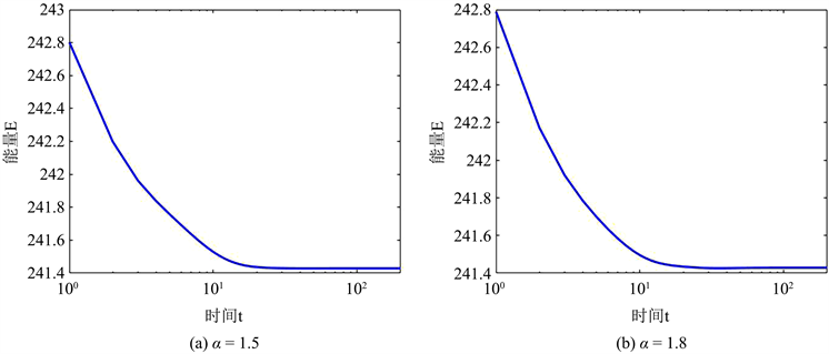
Figure 4. Energy consumption at
图4. 的能量耗损
图3显示了密度场 在 和 时,不同时刻的数值解图像。由图可知,随着时间的推移,微晶相互碰撞并形成晶界,最后充满整个区域并趋于稳态。图4展示了不同 取值下的数值解能量图,验证了算法满足能量递减规律。
5. 结论
本文利用显隐Runge-Kutta方法和傅里叶谱方法求解分数阶守恒Swift-Hohenberg方程,建立了求解该方程的三种高效数值格式,并给出了质量守恒的理论分析。最后,通过数值实验验证了所提出格式的收敛阶和能量递减性。
致谢
由衷感谢华侨大学数学科学学院翟术英老师对本论文提供的支持与帮助!
基金项目
华侨大学2021年大学生创新创业训练项目(S202010385038);华侨大学实验教学与管理改革课题 (SY2021J12)。
文章引用
李 婷,陈筱彦,白怡敏,胡小兵. 分数阶守恒Swift-Hohenberg方程的三种显隐Runge-Kutta方法
Three Explicit and Implicit Runge-Kutta Methods for Fractional Conservation Swift-Hohenberg Equation[J]. 应用数学进展, 2022, 11(04): 2221-2232. https://doi.org/10.12677/AAM.2022.114236
参考文献
- 1. 陈磊, 王猛, 周鹏, 等. 液固相变形核率转变的物理模拟[J]. 铸造技术, 2012, 33(8): 891-894.
- 2. 陈伟, 王宝祥, 冯永平. φ210mm圆坯结晶器电磁场-流场-温度场耦合数值模拟研究[J]. 铸造技术, 2013, 34(4): 458-461.
- 3. Swift, J.B. and Hohenberg, P.C. (1977) Hydrodynamic Fluctuations at the Convective Instability. Physical Review A, 15, 319-328. https://doi.org/10.1103/PhysRevA.15.319
- 4. Zhai, S.Y., Weng, Z.F., Feng, X.L., et al. (2021) Stability and Error Estimate of the Operator Splitting Method for the Phase Field Crystal Equation. Journal of Scientific Computing, 86, Article No. 8. https://doi.org/10.1007/s10915-020-01386-8
- 5. Wang, J.T., Yang, L. and Duan, J.Q. (2020) Recurrent Solutions of a Nonautonomous Modified Swift-Hohenberg Equation. Applied Mathematics and Computation, 379, Article ID: 125270. https://doi.org/10.1016/j.amc.2020.125270
- 6. Zhao, X.P., Liu, B., Zhang, P., et al. (2013) Fourier Spectral Method for the Modified Swift-Hohenberg Equation. Advances in Difference Equations, 2013, Article No. 156. https://doi.org/10.1186/1687-1847-2013-156
- 7. Li, W.J. and Pang, Y.N. (2018) An Iterative Method for Time-Fractional Swift-Hohenberg Equation. Advances in Mathematical Physics, 2018, Article ID: 2405432. https://doi.org/10.1155/2018/2405432
- 8. Zahra, W.K., Nasr, M.A. and Baleanu, D. (2020) Time-Fractional Nonlinear Swift-Hohenberg Equation: Analysis and Numerical Simulation. Alexandria Engineering Journal, 59, 4491-4510. https://doi.org/10.1016/j.aej.2020.08.002
- 9. Alrabaiah, H., Ahmad, I., Shah, K., et al. (2021) Analytical Solution of Non-Linear Fractional Order Swift-Hohenberg Equations. Ain Shams Engineering Journal, 12, 3099-3107.
- 10. Prakasha, D.G., Veeresha, P. and Baskonus, H.M. (2019) Residual Power Series Method for Fractional Swift-Hohenberg Equation. Fractal and Fractional, 3, Article No. 9. https://doi.org/10.3390/fractalfract3010009
- 11. Weng, Z.F., Deng, Y.F., Zhuang, Q.Q., et al. (2021) A Fast and Efficient Numerical Algorithm for Swift-Hohenberg Equation with a Nonlocal Nonlinearity. Applied Mathematics Letters, 118, Article ID: 107170. https://doi.org/10.1016/j.aml.2021.107170
- 12. Elsey, M. and Wirth, B. (2013) A Simple and Efficient Scheme for Phase Field Crystal Simulation. ESAIM: Mathematical Modelling and Numerical Analysis—Modélisation Mathématique et Analyse Numérique, 47, 1413-1432.
- 13. Lee, H.G. (2020) An Efficient and Accurate Method for the Conservative Swift-Hohenberg Equation and Its Numerical Implementation. Mathematics, 8, Article No. 1502. https://doi.org/10.3390/math8091502
- 14. Wang, J.Y. and Zhai, S.Y. (2020) A Fast and Efficient Numerical Algorithm for the Nonlocal Conservative Swift- Hohenberg Equation. Mathematical Problems in Engineering, 2020, Article ID: 7012483. https://doi.org/10.1155/2020/7012483
- 15. Zhang, J. and Yang, X.F. (2019) Numerical Approximations for a New L2-Gradient Flow Based Phase Field Crystal Model with Precise Nonlocal Mass Conservation. Computer Physics Communications, 243, 51-67. https://doi.org/10.1016/j.cpc.2019.05.006
- 16. Kenichi, M., Adrian, A. and Nail, A. (2003) Exact Soliton Solutions of the One-Dimensional Complex Swift-Hohenberg Equation. Physica D: Nonlinear Phenomena, 176, 44-46. https://doi.org/10.1016/S0167-2789(02)00708-X
- 17. 王志林, 纪峰波. 一维复系数Swift-Hohenberg方程的精确解[J]. 兰州大学学报, 2005, 41(3): 110-113.
- 18. 林国广. 非局部二维Swift-Hohenberg方程的惯性流形[J]. 云南大学学报(自然科学版). 2009, 31(4): 334-340.
- 19. 兰天柱. 几类非线性动力系统的动力学行为研究[D]: [硕士学位论文]. 杭州: 杭州师范大学, 2016.
- 20. Lee, H.G. (2017) A Semi-Analytical Fourier Spectral Method for the SH Equation. Computers & Mathematics with Applications, 74, 1885-1896. https://doi.org/10.1016/j.camwa.2017.06.053
- 21. Lee, H.G. (2019) An Energy Stable Method for the SH Equation with Quadratic-Cubic Nonlinearity. Computer Methods in Applied Mechanics and Engineering, 343, 40-45. https://doi.org/10.1016/j.cma.2018.08.019
NOTES
*通讯作者。