Pure Mathematics
Vol.
12
No.
01
(
2022
), Article ID:
48056
,
9
pages
10.12677/PM.2022.121009
一类具退化承载力捕食者–食饵模型的 Hopf分支
王碧君
西北师范大学数学与统计学院,甘肃 兰州
收稿日期:2021年12月4日;录用日期:2022年1月11日;发布日期:2022年1月18日

摘要
本文研究带Holling-II型功能反应的具有退化承载能力的捕食者–食饵模型的稳定性与Hopf分支。首先讨论平衡点的局部渐近稳定性,然后以退化系数 为分支参数,给出Hopf分支存在的条件。最后利用规范型理论和中心流形定理分析Hopf分支的方向及分支周期解的稳定性。
关键词
退化承载力,平衡点,稳定性,Hopf分支

Hopf Bifurcation of a Predator-Prey Model with Degenerate Carrying Capacity
Bijun Wang
College of Mathematics and Statistics, Northwest Normal University, Lanzhou Gansu
Received: Dec. 4th, 2021; accepted: Jan. 11th, 2022; published: Jan. 18th, 2022

ABSTRACT
In this paper, we study the stability and the Hopf bifurcation of apredator-prey model with degenerate carrying capacity with Holling-II type of functional response. Firstly, the local asymptotic stability of the equilibrium point is discussed. Then, the existence condition of the Hopf bifurcation is given by taking the degradation coefficient ρ as the branching parameter. Finally, the direction of the Hopf bifurcation and the stability of its periodic solution are analyzed by means of canonical theory and central manifold theorem.
Keywords:Degradation Capacity, Equilibrium Point, Stability, Hopf Bifurcation

Copyright © 2022 by author(s) and Hans Publishers Inc.
This work is licensed under the Creative Commons Attribution International License (CC BY 4.0).
http://creativecommons.org/licenses/by/4.0/


1. 引言
高原鼠兔是高山草甸生态系统中常见的一种小型狐形哺乳动物。高山草甸是中国和西藏重要的生态系统组成部分。高山草甸提供空气和水净化、生物多样性等重要的生态服务维护,是生态系统中非常重要的组成部分。近几十年里,人们已经观察到忽略高山草甸生态系统对环境造成了一些严重的负面影响 [1] [2] [3]。鼠兔在高山草甸经常被视为害虫,因为它们被观察到与牲畜争夺食物 [4] 并在土壤中制造洞,增加土壤侵蚀 [5] [6] [7]。各种研究表明,高原鼠兔密度高,导致草甸退化 [4] [8]。鼠兔成为植被生长区域减少的原因(通过挖坑和扔土堆),即减少对猎物的承载能力 [9]。刘等人 [10] 在他们的模型中考虑了这一想法,并分析了它的存在性和稳定性以及平衡点的分岔和极限环的存在性。高原鼠兔与高山草甸植被之间存在捕食–被捕食系统的关系,考虑承载能力下降的事实以及植被高度的影响。在文献 [11] 中作者建立了非线性退化承载力的捕食者–食饵模型,模型如下:
(1)
其中x和y分别表示食饵和捕食者种群的密度。参数g代表内禀增长率。 是Holling圆盘函数 [12],代表捕食者的捕食率。参数k代表没有捕食者时的环境容纳量。参数 代表由于高原鼠兔挖洞造成承载力退化系数。d为捕食者种群的自然死亡率,q为转化率, 为捕食者的衰减率,与食饵高度有关。
本文主要研究模型(1)平衡点的稳定性,其次以参数 为分支参数,讨论Hopf分支的存在性。接下来通过中心流行定理,规范型理论和文献 [13] 的方法分析Hopf分支的方向以及分支周期解的稳定性,最后用数值模拟验证所得到的结论。
2. 平衡点的存在性和稳定性
2.1. 平衡点的存在性
对于模型(1),
(i) 总存在平凡平衡点 和半平凡平衡点 。
(ii) 假设(H1) 成立。
当且仅当(H11) ,系统(1)存在一个正常数平衡点 。
当且仅当(H12) ,系统(1)存在两个正常数平衡点 , 其中
2.2. 平衡点的局部稳定性
系统(1)在 处的Jacobi矩阵如下
(2)
下面通过计算系统(1)在每个平衡点处的Jacobi矩阵的特征值,来确定这些平衡点的稳定性。
定理1 (i) 平凡平衡点 是无条件不稳定的。
(ii) 若 成立,则半平凡平衡点 不稳定;否则 是局部渐近稳定的。
证明(i) 系统(1)在平衡点 处的Jacobi矩阵为
(3)
矩阵(3)的特征值为 因此,平衡点 是鞍点,是不稳定的。
(ii) 系统(1)在平衡点 处的Jacobi矩阵为
(4)
若 即 成立,则 是鞍点,不稳定。
若 即 成立,则 渐近稳定。
定理2假设(H1) (H11)成立。若
(H2) 且 ,则 是局部渐近稳定的。
当(H2)中, 且 成立,则 是不稳定的。
当(H1) (H12) (H2)成立,经计算 是鞍点,不稳定。此时 稳定性同上。
证明系统(1)在正常数平衡点 处的Jacobi矩阵为
(5)
其中
矩阵(5)的特征方程为
(6)
其中
则当
即条件(H2)成立时,特征方程(6)的根均具有负实部,进而系统(1)的正常数平衡点 是局部渐近稳定的。反之,特征方程(6)的根不全有负实部且实部不为零,因此正常数平衡点 是不稳定的。
3. Hopf分支的存在性
本节选参数 来研究系统(1)在正常数平衡点 处的Hopf分支的存在性。
引理1假设条件(H1) (H11)成立,则存在 ,使得当 时
(7)
证明 令 。整理得
(8)
且 ,因此,存在 ,使得(7)成立,且 是唯一的。
引理2若条件 ,则模型(1)在 处产生Hopf分支。
证明计算可知:
(9)
下面验证横截性条件。即如果 是特征方程(6)的根,则
表明满足横截性条件。因此,由文献 [14] 的Poincaré-Andronov-Hopf分支定理可得,当 经过 时,系统(1)在 处产生Hopf分支。
4. Hopf分支的方向与稳定性
这一节我们主要研究当 时,模型(1)在 处发生Hopf分支的方向及由分支产生的周期解的稳定性。作变换 ,则平衡点 平移到原点,为了方便,变换后仍用x和y表示 和 ,则模型变为
(10)
对于模型(10)用Taylor展式可化简为
(11)
其中
并且
定义矩阵
其中, ,,可得
则
当 时,有
通过变换 ,模型可重新写为
其中
再用极坐标 系统等价于
对于模型在 处作Taylor展式有
为了得到Hopf分支方向和分支周期解的稳定性,需要计算Liapunov系数 的符号:
所有的偏导数都取值于分支点 ,并且
故 。
因此,可以得到
由Poincaré-Andronov-Hopf分支定理, 和上面关于 的计算可得下列结论。
定理3假设(H1) (H2)成立,则当 时,系统(1)在正平衡点 处产生Hopf分支。若 则Hopf分支方向是亚临界的,分支周期解是渐近稳定的;若 则Hopf分支方向是超临界的,分支周期解是不稳定的。
5. 数值模拟
本节通过数值模拟来验证前面所得到的结果。在系统(1)中选取参数 ,,,,,,,满足系统有正平衡点 经计算, 。当 时,正平衡点 是渐近稳定的,“如图1”所示。当 减小到临界值 ,正平衡点 失稳并且经历Hopf分支,进一步计算可得 ,由定理3,Hopf分支是亚临界的,分支周期解是渐近稳定的。当 时,正平衡点 是不稳定的,且系统(1)存在一个稳定的极限环,“如图2”所示。
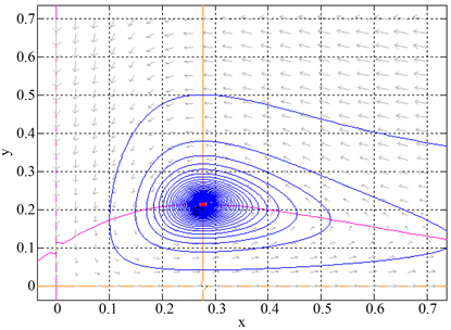
Figure 1. When , the positive equilibrium of system (1) is asymptotically stable
图1. 当 时,系统(1)的正平衡点 是渐近稳定的

Figure 2. When , the positive equilibrium of system (1) is unstable
图2. 当 时,系统(1)的正平衡点 是不稳定的
文章引用
王碧君. 一类具退化承载力捕食者–食饵模型的Hopf分支
Hopf Bifurcation of a Predator-Prey Model with Degenerate Carrying Capacity[J]. 理论数学, 2022, 12(01): 62-70. https://doi.org/10.12677/PM.2022.121009
参考文献
- 1. Zhao, X. and Zhou, X. (1999) Ecological Basis of Alpine Meadow Ecosystem Management in Tibet: Haibei Alpine Meadow Ecosystem Research Station. Ambio, 28, 642-647.
- 2. Wang, X. and Fu, X. (2004) Sustainable Management of Alpine Meadows on the Tibetan Plateau: Problems Overlooked and Suggestions for Change. Ambio, 33,169-171. https://doi.org/10.1579/0044-7447-33.3.169
- 3. Zhou, H., Zhou, L. and Zhao, X. (2006) Stability of Alpine Meadow Ecosystem on the Qinghai-Tibetan Plateau. Chinese Science Bulletin, 51, 320-327. https://doi.org/10.1007/s11434-006-0320-4
- 4. Fan, N.C. (1999) Rodent Pest Management in the Qinghai-Tibet Alpine Meadow Ecosystem. In: Singleton, G.R., Hinds, L.A., Leirs, H. and Zhang, Z., Eds., Ecologically-Based Rodent Management, Australian Centre for International Agricultural Research, Canberra, 213.
- 5. Pech, R., Arthur, A., Zhang, Y. and Hui, L. (2007) Population Dynamics and Responses to Management of Plateau Pikas Ochotonacurzoniae. Journal of Applied Ecology, 44, 615-624. https://doi.org/10.1111/j.1365-2664.2007.01287.x
- 6. Liu, W., Xu, Q., Wang, X., Zhao, J. and Li, Z. (2010) Influence of Burrowing Activity of Plateau Pikas (Ochotonacurzoniae) on Nitrogen in Soils. Acta Theriologica Sinica, 30, 35-44. (In Chinese with English Abstract)
- 7. Guo, Z.G., Zhou, X.R. and Yuan, H. (2012) Effect of Available Burrow Densities of Plateau Pika (Ochotonacurzoniae) on Soil Physicochemical Property of the Bare Land and Vegetation Land in the Qinghai-Tibetan Plateau. Acta Theriologica Sinica, 32, 104-110. (In Chinese with English Abstract) https://doi.org/10.1016/j.chnaes.2012.02.002
- 8. Delibesmateos, M., Smith, A.T., Slobodchikoff, C.N. and Swenson, J.E. (2011) The Paradox of Keystone Species Persecuted as Pests: A Call for the Conservation of Abundant Small Mammals in Their Native Range. Biological Conservation, 144, 1335-1346. https://doi.org/10.1016/j.biocon.2011.02.012
- 9. Wei, X., Li, S., Yang, P. and Cheng, H. (2007) Soil Erosion and Vegetation Succession in Alpine Kobresia Steppe Meadow Caused by Plateau Pika: A Case Study of Nagqu County, Tibet. Chinese Geographical Science, 17, 75-81. https://doi.org/10.1007/s11769-007-0075-0
- 10. Liu, H., Wang, L. and Zhou, H. (2019) Dynamics of a Preda-tor-Prey Model with State-Dependent Carrying Capacity. Discrete and Continuous Dynamical Systems, 24, 4739-4753.
- 11. Amartya Das, G.P. (2021) Samanta: Influence of Environmental Noises on a Prey-Predator Species with Predator-Dependent Carrying Capacity in Alpine Meadow Ecosystem, S0378-4754(21)00264-0.
- 12. Wu, W.J. and Liang, G.W. (1989) Review of Methods Fitting Holling Disk Equation. Natural Enemies of Insects, 11, 96-100.
- 13. Kuznetsov, Y.A. (2013) Elements of Applied Bifurcation Theory. Springer Science-Business Media, New York.
- 14. Hale, J.K. and Kocak, H. (1991) Dynamics and Bifurcations. Springer, New York. https://doi.org/10.1007/978-1-4612-4426-4