Dynamical Systems and Control
Vol.
09
No.
04
(
2020
), Article ID:
37872
,
11
pages
10.12677/DSC.2020.94018
自适应间歇控制下时滞复杂网络的有限时同步
曹娟
南京航空航天大学理学院,江苏 南京
收稿日期:2020年9月4日;录用日期:2020年9月14日;发布日期:2020年9月27日

摘要
由于其在现实生活中的广泛应用,复杂网络的同步问题已经成为了一个热门的话题。本文通过加自适应非周期间歇控制器,研究了一类线性时变时滞耦合复杂网络的有限时同步问题。基于李雅普诺夫稳定性理论以及自适应间歇控制技巧,我们详细证明了在所给的充分条件下,所得有限时同步结论的正确性。此外,我们给出停时的表达式。最后,通过一个时值实例,我们证明了理论结果的合理性。本文的结论对于具体的复杂网络统一适用。
关键词
有限时聚类同步,自适应间歇控制,时变时滞复杂网络
Finite-Time Synchronization of Delayed Complex Networks via Adaptive Intermittent Control
Juan Cao
College of Science, Nanjing University of Aeronautics and Astronautics, Nanjing Jiangsu

Received: Sep. 4th, 2020; accepted: Sep. 14th, 2020; published: Sep. 27th, 2020

ABSTRACT
Due to its wide application in real life, the synchronization of complex networks has become a hot topic. In this article, we investigate the finite-time synchronization for linearly coupled complex networks with time-varying delay by adaptive aperiodically intermittent controllers. Based on the Lyapunov stability theory and the adaptive intermittent control technique, we prove in detail the correctness of the conclusion on finite-time synchronization under the given sufficient conditions. In addition, the expression of settling time is estimated. Last but not least, a numerical example is presented to illustrate the validity of theoretical results. The conclusions of this paper are applicable to the concrete complex networks.
Keywords:Finite-Time Synchronization, Adaptive Intermittent Pinning Control, Delayed Complex Networks

Copyright © 2020 by author(s) and Hans Publishers Inc.
This work is licensed under the Creative Commons Attribution International License (CC BY 4.0).
http://creativecommons.org/licenses/by/4.0/


1. 引言
同步是自然界和社会中普遍存在着的一种现象,例如钟摆的同步摆动、萤火虫的同步发光以及剧场中人们掌声的同步等。复杂网络同步 [1] 的研究已经引起了各个领域研究者们的广泛兴趣,例如通信、工程、物理学、数学、和社会学等。耦合振荡器的同步现象不仅可以解释实际生活中的许多现象 [2],而且具有许多实际应用,例如图像处理 [3]、保密通信 [4] 等。在过去几十年,各种同步种类被广泛研究,例如完全同步、投影同步、相同步、滞后同步、反同步、聚类同步等 [5] - [10]。许多研究者讨论了耦合复杂网络的同步问题,其中含有渐近同步和指数同步的研究 [11] [12]。然而,在实际工程中,人们总是希望使得耦合复杂系统在有限时间内达到同步,理由之一是想避免一些例如信息遗漏的损失。因此,越来越多的人研究耦合复杂网络的有限时同步。例如,文献 [13] 中,作者建立了一个有限时同步准则,该准则可以用于多权重的复杂动态网络。另一个例子是,李等人研究了混合耦合网络的有限时同步问题 [14]。
值得注意的是,之前的工作中已经提出了许多种控制策略,例如牵制控制、基于观测者控制、样本数据控制、反馈控制、自适应控制、间歇控制、脉冲控制等 [15] - [21]。由于间歇控制具有不连续的工作时间并且可以减少控制成本和传输信息的数量,它很容易在工程中得以使用。此外,自适应控制可以通过提前设计好的办法来自动地调节其增益。因此,一些学者将二者相结合来设计控制器。间歇控制可以是周期的或非周期的,周期间歇控制意味着每个控制阶段固定,而非间歇控制的控制阶段不固定。众所周知,时滞频繁地出现在工程、通信、生物系统等现实系统中,它们可能会导致Hopf分支、混沌等不理想的动力学行为 [22],所以考虑带有时滞的复杂网络很有必要。对比于复杂网络的渐近同步和指数同步,有限时同步不仅具有更快的收敛速度,而且更符合实际应用的需求。研究有限时同步可以使系统具有更好的抗干扰性以及鲁棒性。有限时同步有助于确定网络在有限时间范围内实现同步,这意味着通过设计适当的控制器,受控系统的轨道可以在有限时间内趋于平衡状态。基于之前的相关文献,本文研究自适应非周期间歇控制下时变时滞复杂网络的有限时同步问题。
2. 初步
2.1. 模型描述
定义一个加权有向图 ,其点集为 ,边集为 。定义一个加权邻
接矩阵 ,其中每个元素 非负,设对于所有 ,。在一个有向图中,若任意两个
不同的节点之间总存在一条有向路径将其连接,这个有向图就称为强连通。
考虑如下由有向图G上N个节点组成的具有时变时滞的线性耦合系统,
(1)
其中 是系统的状态向量, 代表系统动力学节点内部的时变时滞, 并且 。激活函数 连续, 代表耦合权重,当且仅当图G中节点i和节点j之间无连接时 。
我们把上述的系统(1)看作驱动系统,参照系统(1),可以给出对应的响应系统为
(2)
其中 , 指响应系统第i个节点的控制输入。
将同步误差向量记为 ,根据驱动系统(1)以及相应的响应系统(2),我们有如下的误差系统
为了保证驱动响应系统(1)和(2)可以在有限时间内实现同步现象,我们设计如下的定量自适应非周期间歇控制器,
(3)
其中 ,,,。 为一个时间跨度, 。 指工作时间,而 为休息时间。 为第m个控制宽度,而 为第m个休息宽度。 是一个量化器,其中 ,,并且 [23] 给定如下
(4)
其中 ,,。根据文献 [23],存在 ,使得 。而且自适应
法则如下
其中 。
2.2. 数学准备
在这一部分,我们给出一个假设,两个定义以及一个引理,以帮助获得本文的主要结果。
假设1 对于函数f,假设存在正常数 ,使得
;对于内部耦合矩阵 ,有 。
定义1 驱动系统(1)和响应系统(2)称为实现有限时同步,如果对于一个恰当的自适应非周期间歇控制
器(3),存在一个常数 ,使得 并且当 时,有 ,其中, 。
定义2 [24] 对于非周期间歇控制,定义 。显然, ,并且 时,休息
宽度为0,该控制变为连续控制输入。
引理1 [25] 若函数 连续且在 上非负,满足如下条件:
其中 ,,。若存在定义2当中的数 ,则有如下不等式成立
其中T是如下给出的停时:若 ,则 ;若 ,则T是方程 的最小解。
3. 主要结论
在这个部分,我们给出一个充分性准则以及一个推论,通过施加一个定量自适应非周期间歇控制器(3)实现驱动系统(1)和响应系统(2)之间的有限时同步。
定理1 假设有向图 强连通且满足假设1,则驱动系统(1)和响应系统(2)可以在有限时间内实现同步,若如下条件成立:对于 ,
1) 控制器 中存在正常数 使得 ;
2) 成立不等式 ,,其中 ,,,, 与文献 [26] 中定理2中的定义相同, ,
并且停时为
其中 是方程 的最小解。
证明 定义李雅普诺夫泛函 。因此,可以得 。
根据文献 [26] 中的定理2.2,由 强连通,我们可以有 。因此,根据(3)式及假设1,当 时,我们有
(5)
由量化器的性质有 ,则对 ,有 ,则 ,。
根据(3)式和假设1,有
(6)
(7)
将(6)和(7)式代入(5)式,可以得出
因为 ,,,所以
类似地,当 时,有
概括两者
由引理1及条件2可以算出
并且停时为
其中 是方程 的最小解。因此,根据定义1,驱动系统(1)和响应
系统(2)可以实现有限时同步。这样就完成了证明。
若参数 ,自适应非周期间歇控制器就会变成一个连续控制器,定理1便会变成如下的推论。
推论1 假设定理1的其余条件满足并且条件(2)改成如下的条件(2’),则驱动系统(1)和响应系统(2)可以在有限时间内实现同步,
(2’)成立不等式 ,
并且停时为 ,其中 和 与定理相同。
4. 数值模拟
蔡少棠教授于1983年提出的蔡电路,是当前混沌电路中最具代表性的一种。其典型的电路结构已经使其成为一个无处不在的现实世界混沌系统的例子。通过电磁学定律的应用,蔡电路可以准确地建模出。近期,蔡电路模型被作为一种原型电子系统而广泛研究。本部分给出蔡电路的模型,以阐明有限时同步
结论的有效性。单个蔡电路的模型 [27] 为: ,各字母的实际含义可以参考文献 [27],并且 ,其中 为常数。
在这个模型的基础上加上时变时滞及耦合效果后变为如下形式:
(8)
其中 ,,,,,,, 且 ,。 为节点内部发生的时变时滞且 。我们可以将系
统(8)看作驱动系统,相应的受控响应系统为:
(9)
(10)
, 为常数。 ,,,,,。 按(4)来定义并且自适应法则为
其中 为正常数。结合(8)和(9)有如下的误差系统:
(11)
其中 ,。考虑在一个有向强连通图(图1)上的蔡电路模型,
有向图的邻接矩阵为
![]()
Figure 1. A strongly connected digraph with 4 nodes
图1. 具有4个节点的一个强连通有向图
系统参数选取为 ,,,,,,,,,,,,,,,,,,,,,,,,,,,,,,,,,,,,,,。
通过计算,可得出停时为 。此外,我们可以知道定理1的所有条件成立。图2给出了自适应法则 随时间的演变,其中,绿色曲线表示 ,蓝色曲线表示 ,黑色曲线表示 ,紫色曲线表示 。从中我们可以看到当停时达到以后,所有的自适应法则都逼近于某个常数。图3展示的是带有定量自适应非周期间歇控制器(10)的同步误差轨道(11),其中每一个曲线分别表示一个误差 ,,。不管误差状态的轨道一开始的变化有多复杂,在时间趋近于停时时,误差的状态都会逼近于0,而当时间超过停时以后,所有的误差的状态一直恒为0。从图3可以看出具有时变时滞的耦合蔡电路模型可以实现有限时同步,这证实了我们所提出的理论结果是正确的。
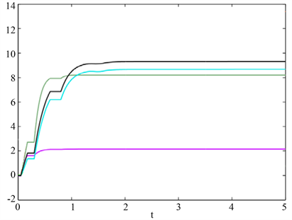
Figure 2. Evolution of adaptive laws with ,,,
图2. 自适应法则 的演变,并且 ,,,

Figure 3. Trajectories of synchronous error system (11)
图3. 同步误差系统(11)的轨道
5. 结论
本文详细地研究了一类具有时变时滞的复杂网络的有限时同步问题。我们考虑强连通的网络拓扑、非线性的激活函数以及内部耦合的网络结构。基于李雅普诺夫稳定性理论和有限时控制技巧,我们设计出一种定量非周期间歇控制来帮助该网络实现有限时同步。最近几十年中,由于采用有限精度算法的数字计算机的广泛使用,控制系统的信号量化研究得到了许多关注。在定量自适应非周期间歇控制中,信号在传输之前得以量化。对比连续控制方案,间歇控制不仅可以节约控制成本,而且可以帮助减少信道拥塞。最后,我们通过给出一个在蔡氏电路模型上的应用来体现本文的有限时同步结论的合理性。进一步,我们还可以研究非强连通的网络拓扑情况下,如何通过间歇控制来实现该网络的有限时同步。
文章引用
曹 娟. 自适应间歇控制下时滞复杂网络的有限时同步
Finite-Time Synchronization of Delayed Complex Networks via Adaptive Intermittent Control[J]. 动力系统与控制, 2020, 09(04): 185-195. https://doi.org/10.12677/DSC.2020.94018
参考文献
- 1. Wang, Z.X., Jiang, G.P., Yu, W.W., He, W.L., Cao, J.D. and Xiao, M. (2017) Synchronization of Coupled Heterogeneous Complex Networks. Journal of the Franklin Institute, 354, 4102-4125.
https://doi.org/10.1016/j.jfranklin.2017.03.006 - 2. Mirollo, R.E. and Strogatz, S.H. (1990) Synchronization of Pulse-Coupled Biological Oscillators. SIAM Journal on Applied Mathematics, 50, 1645-1662.
https://doi.org/10.1137/0150098 - 3. Wei, G.W. and Jia, Y.Q. (2002) Synchronization-Based Image Edge Detection. Europhysics Letters, 59, 814-819.
https://doi.org/10.1209/epl/i2002-00115-8 - 4. Nechifora, A., Albub, M., Hairc, R. and Terzijaa, V. (2015) A Flexible Platform for Synchronized Measurements, Data Aggregation and Information Retrieval. Electric Power Systems Research, 120, 20-31.
https://doi.org/10.1016/j.epsr.2014.11.008 - 5. Liu, J., Li, L.L. and Fardoun, H.M. (2020) Complete Synchronization of Coupled Boolean Networks with Arbitrary Finite Delays. Frontiers of Information Technology & Electronic Engineering, 21, 281-293.
https://doi.org/10.1631/FITEE.1900438 - 6. Ren, L. and Zhang, G.S. (2019) Adaptive Projective Synchronization for a Class of Switched Chaotic Systems. Mathematical Methods in the Applied Sciences, 42, 6192-6204.
https://doi.org/10.1002/mma.5714 - 7. Aguirre, L.A. and Freitas, L. (2018) Control and Observability Aspects of Phase Synchronization. Nonlinear Dynamics, 91, 2203-2217.
https://doi.org/10.1007/s11071-017-4009-9 - 8. Cai, S.M., Zhou, F.L. and He, Q.B. (2019) Fixed-Time Cluster Lag Synchronization in Directed Heterogeneous Community Networks. Physica A: Statistical Mechanics and Its Applications, 525, 128-142.
https://doi.org/10.1016/j.physa.2019.03.033 - 9. Zhang, C.L., Deng, F.Q., Zhang, W.F., Hou, T. and Yang, Z.W. (2019) Anti-Synchronization and Synchronization of Coupled Chaotic System with Ring Connection and Stochastic Perturbations. IEEE Access, 7, 76902-76909.
https://doi.org/10.1109/ACCESS.2019.2921661 - 10. Gan, Q., Xiao, F., Qin, Y. and Yang, J. (2019) Fixed-Time Cluster Synchronization of Discontinuous Directed Community Networks via Periodically or Aperiodically Switching Control. IEEE Access, 7, 83306-83318.
https://doi.org/10.1109/ACCESS.2019.2924661 - 11. Wang, P.F., Zou, W.Q., Su, H. and Feng, J.Q. (2019) Exponential Synchronization of Complex-Valued Delayed Coupled Systems on Networks with Aperiodically On-Off Coupling. Neurocomputing, 369, 155-165.
https://doi.org/10.1016/j.neucom.2019.08.077 - 12. Guo, Z.Y., Gong, S.Q., Yang, S.F. and Huang, T.W. (2018) Global Exponential Synchronization of Multiple Coupled Inertial Memristive Neural Networks with Time-Varying Delay via Nonlinear Coupling. Neural Networks, 108, 260-271.
https://doi.org/10.1016/j.neunet.2018.08.020 - 13. Qiu, S.-H., Huang, Y.-L. and Ren, S.-Y. (2018) Finite-Time Synchronization of Multi-Weighted Complex Dynamical Networks with and without Coupling Delay. Neurocomputing, 275, 1250-1260.
https://doi.org/10.1016/j.neucom.2017.09.073 - 14. Li, D. and Cao, J. (2015) Finite-Time Synchronization of Coupled Networks with One Single Time-Varying Delay Coupling. Neurocomputing, 166, 265-270.
https://doi.org/10.1016/j.neucom.2015.04.013 - 15. Yu, W.W., Chen, G.R., Lu, J.H. and Kurths, J. (2013) Synchronization via Pinning Control on General Complex Networks. SIAM Journal on Control and Optimization, 51, 1395-1416.
https://doi.org/10.1137/100781699 - 16. Wang, Q.Z., He, Y., Tan, G.Z. and Wu, M. (2017) Observer-Based Periodically Intermittent Control for Linear Systems via Piecewise Lyapunov Function Method. Applied Mathematics and Computation, 293, 438-447.
https://doi.org/10.1016/j.amc.2016.08.042 - 17. Ge, C., Wang, H., Liu, Y. and Park, J.H. (2017) Further Results on Stabilization of Neural-Network-Based Systems Using Sampled-Data Control. Nonlinear Dynamics, 90, 2209-2219.
https://doi.org/10.1007/s11071-017-3796-3 - 18. Lv, X., Li, X., Cao, J. and Duan, P. (2018) Exponential Synchronization of Neural Networks via Feedback Control in Complex Environment. Complexity, 2018, Article ID: 4352714.
- 19. Li, Q.-N., Yang, R.-N. and Liu, Z.-C. (2017) Adaptive Tracking Control for a Class of Nonlinear Non-Strict-Feedback Systems. Nonlinear Dynamics, 88, 1537-1550.
https://doi.org/10.1007/s11071-016-3327-7 - 20. Li, L.L., Tu, Z.W., Mei, J. and Jian, J.G. (2016) Finite-Time Synchronization of Complex Delayed Networks via Intermittent Control with Multiple Switched Periods. Nonlinear Dynamics, 85, 375-388.
https://doi.org/10.1007/s11071-016-2692-6 - 21. Yi, C.B., Feng, J.W., Wang, J.Y., Xu, C. and Zhao, Y. (2017) Synchronization of Delayed Neural Networks with Hybrid Coupling via Partial Mixed Pinning Impulsive Control. Applied Mathematics & Computation, 312, 78-90.
https://doi.org/10.1016/j.amc.2017.04.030 - 22. Liang, J.L., Wang, Z.D. and Liu, X.H. (2009) State Estimation for Coupled Uncertain Stochastic Networks with Missing Measurements and Time-Varying Delays: The Discrete-Time Case. IEEE Transactions on Neural Networks, 20, 781-793.
https://doi.org/10.1109/TNN.2009.2013240 - 23. Xu, C., Yang, X., Lu, J., Feng, J., Alsaadi, F.E. and Hayat, T. (2017) Finite-Time Synchronization of Networks via Quantized Intermittent Pinning Control. IEEE Transactions on Cybernetics, 48, 3021-3027.
https://doi.org/10.1109/TCYB.2017.2749248 - 24. Liu, X.W. and Chen, T.P. (2015) Synchronization of Linearly Coupled Networks with Delays via Aperiodically Intermittent Pinning Control. IEEE Transactions on Neural Networks and Learning Systems, 26, 2396-2407.
https://doi.org/10.1109/TNNLS.2014.2383174 - 25. Liu, M., Jiang, H. and Hu, C. (2017) Finite-Time Synchronization of Delayed Dynamical Networks via Aperiodically Intermittent Control. Journal of the Franklin Institute—Engineering and Applied Mathematics, 354, 5374-5397.
https://doi.org/10.1016/j.jfranklin.2017.05.030 - 26. Li, M.Y. and Shuai, Z.S. (2010) Global-Stability Problem for Coupled Systems of Differential Equations on Networks. Journal of Differential Equations, 248, 1-20.
https://doi.org/10.1016/j.jde.2009.09.003 - 27. Chua, L.O. (1993) Chaos Synchronization in Chua’s Circuit. Journal of Circuits, Systems and Computers, 3, 93-108.
https://doi.org/10.1142/S0218126693000071