Advances in Applied Mathematics
Vol.07 No.05(2018), Article ID:25061,10
pages
10.12677/AAM.2018.75068
High Order Discontinuous Galerkin Methods with Differential Transform Strategy
Haiyan Yu, Xiufang Wang, Gang Li
School of Mathematics and Statistics, Qingdao University, Qingdao Shandong
![]()
Received: Apr. 30th, 2018; accepted: May 16th, 2018; published: May 25th, 2018

ABSTRACT
In this paper, based on the differential transform strategy, we introduce high order full discrete discontinuous Galerkin methods for one-dimensional hyperbolic conservation laws. Compared with the standard discontinuous Galerkin methods, the current methods enjoy the following advantages including low storage as well as keeping arbitrary high order accuracy in time. In comparison with the ADER methods, the resulting methods avoid the complicated Cauchy-Kowalewski procedure and the coding is easy at the same time. In addition, numerical results also indicate that the resulting methods enjoy genuine high order accuracy for smooth solutions, and keep steep discontinuity transition.
Keywords:Hyperbolic Conservation Laws, Discontinuous Galerkin Methods, Differential Transformation, High Order Accuracy, Full Discrete
基于微分变换策略的全离散间断Galerkin方法
于海燕,王秀芳,李刚
青岛大学,数学与统计学院,山东 青岛
![]()
收稿日期:2018年4月30日;录用日期:2018年5月16日;发布日期:2018年5月25日

摘 要
在本文中,针对一维双曲守恒律方程,我们基于微分变换策略提出了一种高阶全离散间断Galerkin方法。与传统间断Galerkin方法相比较,该方法的主要特点为存储量较小,在时间上能够到达任意高阶精度。与ADER方法相比较,避免了复杂的Cauchy-Kowalewski步骤,同时程序编写简单。数值结果表明该方法具有高阶精度,针对间断解保持高分辨率。
关键词 :双曲守恒律,间断Galerkin方法,微分变换,高阶精度,全离散

Copyright © 2018 by authors and Hans Publishers Inc.
This work is licensed under the Creative Commons Attribution International License (CC BY).
http://creativecommons.org/licenses/by/4.0/


1. 引言
在本文中,考虑双曲守恒律
的高阶数值方法。间断Galerkin (DG)方法作为一种高阶方法首先由Reed和Hill [1] 于1973年在求解中子输运问题时提出。上个世纪90年代,Cockburn,Chi-Wang Shu等人 [2] [3] [4] [5] 提出了基于Runge-Kutta时间离散方法的Runge-Kutta DG (RKDG)方法,并将该方法成功应用于双曲守恒律方程。DG方法使用分段间断多项式空间作为试探和检验函数空间,并结合了有限元方法和有限体积格式的优点,特别易于处理复杂边界和边值问题,拥有灵活处理间断的能力,同时又适合自适应算法与并行策略,因此在计算流体力学领域得到了广泛应用 [6] - [17] 。关于DG方法的历史回顾与最新进展见文献 [18] [19] [20] 。传统的RKDG方法为显格式,其优点在于每个时间步长计算中不需要求解大规模线性代数方程组。但是,传统RKDG方法作为一种高精度方法,由于中间步的存在,导致存储量较高。此外,RKDG方法因为使用Gauss数值求积,所以计算成本非常高。
近年来以ADER方法 [21] 为代表的时–空任意高阶方法取得了长足进步。ADER方法是一类基于有限体积积分的具有高阶精度的数值方法。在ADER方法框架内,在间断面处对时间进行Taylor展开,人们通常使用Cauchu-Kowalewski步骤(又称为Lax-Wendroff步骤) [22] 将时间导数项转换为时间导数项,然后分别求解由展开式中的各个部分所构造的黎曼问题。但是Cauchu-Kowalewski步骤非常复杂,计算成本较高,同时编程复杂。
在本文中,针对双曲守恒律基于微分变换策略提出了高阶全离散DG方法。该DG方法是单步、显式的和全离散的,从而避免了存储量过高的缺点。此外微分变换策略较之Cauchu-Kowalewski过程更加简洁,程序编写简单。更进一步,因为数值解关于时间、空间皆表示为多项式,故可以使用精确积分,从而避免了计算成本较高的Gauss积分,节约了计算成本,因此更加适应实际问题的需求。
2. 微分变换简介
基于微分方程本身以得到方程解的时–空Taylor级数系数的递推关系,这种策略被称为微分变换(differential transformation) [23] 。与ADER方法中所用到的Cauchy-Kowalewski (C-K)技巧或者Lax-Wendforr技巧相比较,微分变换策略显得更简单,程序编写更加简洁。但是,并非所有方程都能够使用微分变换策略。目前,可以确定的是针对浅水波方程、欧拉方程可以使用微分变换策略 [24] 。
以一维Burgers方程的初值问题
为例解释如何借助微分变换策略求解微分方程。
记Burgers方程为
(1)
其中 为流通量。首先得到 ,即把初始条件表示为 。然后,我们把未知函数 以及流通量 都展成时–空Taylor级数
(2)
其中 。
将(2)中两个等式代入方程(1),得到
调整下求和符号中的下标,得到
比较上式两端,得到如下递推关系
(3)
借助于已有的 ,并利用递推公式(3),可以得到解 的时–空Taylor级数展开式。
针对方程组,可以逐方程地借助微分变换策略来求解微分方程。
3. 一维问题的全离散DG方法
考虑非线性双曲守恒律方程
(4)
首先将方程(4)两端同乘以检验函数 ,并在时–空单元 上积分,然后利用分部积分得到:
对于积分 ,采用简单的Lax-Friedrichs数值流通量来逼近,即
这里 ,其中 为雅克比矩阵 的特征值,并且最大值是在整个计算区域来取。
最后,得到全离散DG方法:对于 , 满足
由于 , 均表示为关于x,t的多项式,所以对于积分采用精确积分,从而避免了计算成本较高的Gauss积分。
4. 数值结果
在本节中,通过数值实验来展示所提出的DG方法的良好性能。针对所有数值算例,我们分别将时间与空间取为二次多项式与四次多项式(即分别取 ,此时取 。或者 ,同时取 )作为基函数。重力常数g取为9.812。
4.1. 精度测试
借助具有光滑解的算例来测试方法的精度阶。考虑线性对流方程:
将该算例计算至 ,同时将方法的数值误差与精度阶分别展示于表1。从表中,可以很明显地发现该方法拥有预期的高阶精度。
4.2. 线性对流方程
借助带有间断解的算例来测试方法能否保持高分辨率

Table 1. Third-order method error and precision order
表1. 三阶方法的误差和精度阶
其中
这里,取 , 。参数取作 , , , , 。
基于带有100个单元的网格,将该算例计算至 ,同时将数值结果展示于图1。我们从图中发现数值结果能够同精确解保持很好的一致性,且保持高分辨率。
4.3. Burgers方程
接下来,测试该方法针对强间断问题能否保持高分辨率,考虑一维Burgers方程:
考虑初始条件
该问题在 时刻会产生激波。接下来考虑另一种初始条件
该初值问题会在左侧产生稀疏波,右侧产生激波。我们把以上两种初值问题的数值结果展示于图2并与精确解相比较。很显然数值结果保持陡峭的间断过渡,从而说明该方法对于间断解同样保持高分辨率。
4.4. 浅水波方程
首先以水动力学中的一维浅水波方程
为例来考虑方程组情形。
其中h,u分别表示水深,深度平均速度。g表示重力常数。
考虑浅水波方程中经典的Riemann问题,又称溃坝问题 [25] ,其初始条件具有以下情形:
其中 为大坝位置, 与 分别表示大坝左右两侧的水体深度与速度。
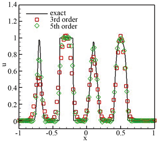
Figure 1. The numerical result of the linear convection equation at time t = 2. Grid n = 100
图1. 线性对流方程在t = 2时刻的数值结果。网格n = 100
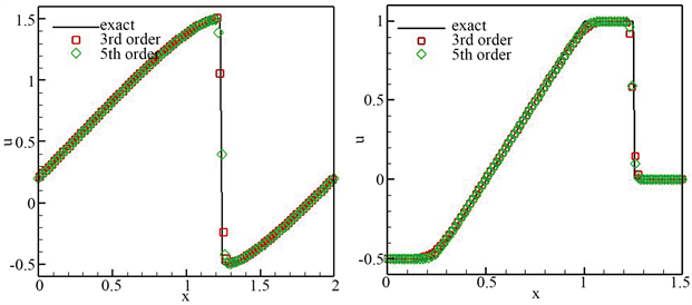
Figure 2. Numerical results for the Burgers equation, grid n = 100. Left: t = 1.5/π, right: t = 0.5
图2. Burgers方程的数值结果,网格n = 100。左:t = 1.5/π,右:t = 0.5
我们考虑以下几种不同的初始条件:
4.4.1. 情形一
初始条件为
计算区域为区间 。计算该算例至 ,同时将计算结果展示于图3并与精确解相比较。数值结果表明数值结果与精确解保持一致,同时保持非振荡性质。
4.4.2. 情形二
初始条件如下:
计算区域为 。将 时刻的数值结果展示于图4。数值结果表明数值结果与精确解保持一致。
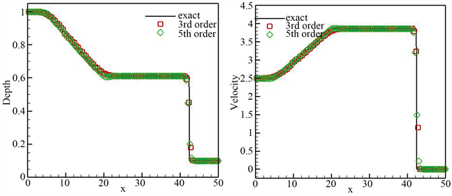
Figure 3. At the time t = 7, the result of the grid is n = 100. Water depth (left) and speed (right)
图3. 在t = 7时刻的数值结果,网格n = 100。水体深度(左)与速度(右)
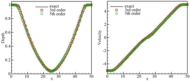
Figure 4. At the time t = 2.5, the result of the grid is n = 100. Water depth (left) and speed (right)
图4. 在t = 2.5时刻的数值结果,网格n = 100。水体深度(左)与速度(右)
4.5. 欧拉方程
考虑空气动力学中的可压缩欧拉方程
其中ρ为密度,u为速度,E表示总能量,p是压力,且与总能量有如下关系
其中γ为绝热比常数,在本文中取作 。
4.5.1. Sod问题
初始条件如下
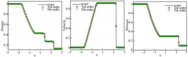
Figure 5. The numerical result of Sod problem at t = 1.3, grid n = 200. From left to right: density, speed, pressure. nx = 200
图5. Sod问题在t = 1.3时刻的数值结果,网格n = 200。从左向右:密度,速度,压力。nx = 200
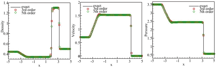
Figure 6. Lax problem numerical results at t = 1.3. Grid n = 200. From left to right: density, speed, pressure
图6. Lax问题在t = 1.3时刻的数值结果。网格n = 200。从左向右:密度,速度,压力
计算区域为[−5, 5]。将 时刻的数值结果展示于图5。数值结果保持很好的分辨率。
4.5.2. Lax问题
初始条件如下
计算区域为[−5, 5]。将时刻 的计算结果展示于图6。数值结果保持很好的间断过度。
5. 结论
在本文中,基于微分变换策略提出了一种高阶全离散间断Galerkin方法。该方法的存储量较小,程序编写简单。针对单个方程以及方程组,开展了广泛数值实验。数值结果表明该方法针对光滑问题具有高阶精度,同时针对间断解拥有高分辨率。
致谢
本研究得到国家自然科学基金项目(11771228)的资助。
文章引用
于海燕,王秀芳,李 刚. 基于微分变换策略的全离散间断Galerkin方法
High Order Discontinuous Galerkin Methods with Differential Transform Strategy[J]. 应用数学进展, 2018, 07(05): 574-583. https://doi.org/10.12677/AAM.2018.75068
参考文献
- 1. Reed, W.H. and Hill, T.R. (1973) Trigangular Mesh Methods for the Neutron Transportation Equation. Technical Report LA-UR-73-479, Los Alamos Scientific Laboratory.
- 2. Cockburn, B. and Shu, C.-W. (1989) TVB Runge-Kutta Local Projection Discontinuous Galerkin Finite Element Method for Conservation Laws for Conservation Laws II: General Framework. Mathematics of Computation, 52, 411-435.
- 3. Cockburn, B., Lin, S.Y. and Shu, C.-W. (1989) TVB Runge-Kutta Local Projection Discontinuous Galerkin Finite Element Method for Conservation Laws for Conservation Laws III: One-Dimensional Systems. Journal of Com-putational Physics, 84, 90-113.
https://doi.org/10.1016/0021-9991(89)90183-6 - 4. Cockburn, B., Hou, S. and Shu. C.-W. (1990) The TVB Runge-Kutta Local Projection Discontinuous Galerkin Finite Element Method for Conservation Laws for Conser-vation Laws IV: The Multidimensional Case. Mathematics of Computation, 54, 545-581.
- 5. Cockburn, B. and Shu, C.-W. (1998) The Runge-Kutta Discontinuous Galerkin Method for Conservation Laws V: Multidimensional Systems. Journal of Computational Physics, 141, 199-224.
https://doi.org/10.1006/jcph.1998.5892 - 6. Aizinger, V. and Dawson, C. (2002) A Discontinuous Galerkin Method for Two-Dimensional Flow and Transport in Shallow Water. Advances in Water Resources, 25, 67-84.
https://doi.org/10.1016/S0309-1708(01)00019-7 - 7. Nair, R.D., Thomas, S.J. and Loft, R.D. (2005) A Discontinuous Galerkin Global Shallow Water Model. Monthly Weather Review, 133, 876-888.
https://doi.org/10.1175/MWR2903.1 - 8. Schwanenberg, D. and Harms, M. (2004) Discontinuous Galerkin Finite-Element Method for Transcritical Two-Dimensional Shallow Water Flow. Journal of Hydraulic Engineering, 130, 412-421.
https://doi.org/10.1061/(ASCE)0733-9429(2004)130:5(412) - 9. Fagherazzi, S., Rasetarinera, P., Hussaini, Y.M. and Furbish, D.J. (2004) Numerical Solution of the Dam-Break Problem with a Discontinuous Galerkin Method. Journal of Hydraulic Engineering, 130, 532-539.
https://doi.org/10.1061/(ASCE)0733-9429(2004)130:6(532) - 10. Eskilsson, C. and Sherwin, S.J. (2004) A Triangular Spec-tral/hp Discontinuous Galerkin Method for Modelling 2D Shallow Water Equations. International Journal for Numerical Methods in Fluids, 45, 605-623.
https://doi.org/10.1002/fld.709 - 11. Aureli, F., Maranzoni, A., Mignosa, P. and Ziveri, C.A. (2008) Weighted Surface-Depth Gradient Method for the Numerical Integration of the 2D Shallow Water Equations with Topography. Advances in Water Resources, 31, 962-974.
https://doi.org/10.1016/j.advwatres.2008.03.005 - 12. Ern, A., Piperno, S. and Djadel, K. (2008) A Well-Balanced Runge-Kutta Discontinuous Galerkin Method for the Shallow-Water Equations with Flooding and Drying. International Journal for Numerical Methods in Fluids, 58, 1-25.
https://doi.org/10.1002/fld.1674 - 13. Canestrelli, A., Siviglia, A., Dumbser, M. and Toro, E.F. (2009) Well-Balanced High-Order Centred Schemes for Non-Conservative Hyperbolic Systems. Applications to Shallow Water Equations with Fixed and Mobile Bed. Advances in Water Resources, 32, 834-844.
https://doi.org/10.1016/j.advwatres.2009.02.006 - 14. Xing, Y.L., Zhang, X.X. and Shu, C.-W. (2010) Positivity-Preserving High Order Well-Balanced Discontinuous Galerkin Methods for the Shallow Water Equations. Advances in Water Resources, 33, 1476-1493.
https://doi.org/10.1016/j.advwatres.2010.08.005 - 15. Kesserwani, G., Liang, Q., Vazquez, J. and Mosé, R. (2010) Well-Balancing Issues Related to the RKDG2 Scheme for the Shallow Water Equations. International Journal for Numerical Methods in Fluids, 62, 428-448.
- 16. Benkhaldoun, F., Elmahi, I. and Sea, M. (2010) A New Finite Volume Method for Flux-Gradient and Source-Term Balancing in Shallow Water Equations. Computer Methods in Applied Mechanics and Engineering, 199, 3224-3335.
https://doi.org/10.1016/j.cma.2010.07.003 - 17. Kesserwani, G. and Liang, Q.H. (2010) A Discontinuous Galerkin Algorithm for the Two-Dimensional Shallow Water Equations. Computer Methods in Applied Mechanics and Engineering, 199, 3356-3368.
https://doi.org/10.1016/j.cma.2010.07.007 - 18. Cockburn, B., Karniadakis, G. and Shu, C.-W. (2000) The Development of Discontinuous Galerkin Methods. In: Cockburn, B., Karniadakis, G. and Shu, C.-W., Eds., Discontinuous Galerkin Methods: Theory, Computation and Applications, Lecture Notes in Computational Science and Engineering, Part I: Overview, Springer, Berlin, 3-50.
https://doi.org/10.1007/978-3-642-59721-3_1 - 19. Shu, C.-W. (2016) High Order WENO and DG Methods for Time-Dependent Convection-Dominated PDEs: A Brief Survey of Several Recent Developments. Journal of Computational Physics, 316, 598-613.
https://doi.org/10.1016/j.jcp.2016.04.030 - 20. Shu, C.-W. (2013) A Brief Survey on Discontinuous Galerkin Ethods in Com-putational Fluid Dynamics. Advances in Mechanics, 43, 541-554.
- 21. Toro, E.F., Millington, R.C. and Nejad, L.A.M. (2001) To-wards Very High Order Godunov Schemes. In: Toro, E.F., Ed., Godunov Methods. Theory and Applications, Edited Review, Kluwer Academic Publishers, Dordrecht, 907-940.
https://doi.org/10.1007/978-1-4615-0663-8_87 - 22. Dumbse, M., Kaser, M., Titarev, V.A. and Toro, E.F. (2007) Quadra-ture-Free Non-Oscillatory Finite Volume Schemes on Unstructured Meshes for Nonlinear Hypobolic Systems. Journal of Computa-tional Physics, 226, 204-243.
https://doi.org/10.1016/j.jcp.2007.04.004 - 23. Ayaz, F. (2004) Solutions of the System of Differential Equations by Differential Transform Method. Applied Mathematics and Computation, 147, 547-567.
https://doi.org/10.1016/S0096-3003(02)00794-4 - 24. Norman, M.R. and Finkel, H. (2012) Multi-Moment ADER-Taylor Methods for Systems of Conservation Laws with Source Terms in One Dimension. Journal of Computational Physics, 231, 6622-6642.
https://doi.org/10.1016/j.jcp.2012.05.029 - 25. Vukovic, S. and Sopta, L. (2002) ENO and WENO Schemes with the Exact Conservation Property for One-Dimensional Shallow Water Equations. Journal of Computational Physics, 179, 593-621.
https://doi.org/10.1006/jcph.2002.7076