Advances in Applied Mathematics
Vol.
08
No.
03
(
2019
), Article ID:
29317
,
12
pages
10.12677/AAM.2019.83057
Conjugate Gradient Method for Norm Problems
Jiaming Zhan, Caiying Wu*
School of Mathematical Sciences, Inner Mongolia University, Hohhot Inner Mongolia

Received: Feb. 28th, 2019; accepted: Mar. 13th, 2019; published: Mar. 20th, 2019

ABSTRACT
A new model is proposed for sparse signal reconstruction. We smooth our model by smoothing absolute value function. Then we use a new tri-term conjugate gradient method to restore sparse signal. The effect of different parameters on sparse signal recovery is tested. The numerical results show that our algorithm is efficient.
Keywords:Sparse Signal Recovery, Conjugate Gradient Method, Norm, Global Convergence

求解基于 范数问题的共轭梯度法
詹佳明,乌彩英*
内蒙古大学数学科学学院,内蒙古 呼和浩特

收稿日期:2019年2月28日;录用日期:2019年3月13日;发布日期:2019年3月20日

摘 要
本文针对稀疏信号的重构问题提出新的函数模型,通过光滑化绝对值函数光滑我们的模型,基于三项共轭梯度法对稀疏信号进行恢复,并试验了不同参数值对稀疏信号恢复效果的影响,数值实验表明本文算法的数值有效性。
关键词 :稀疏信号恢复,三项共轭梯度法, 范数,全局收敛性

Copyright © 2019 by author(s) and Hans Publishers Inc.
This work is licensed under the Creative Commons Attribution International License (CC BY).
http://creativecommons.org/licenses/by/4.0/


1. 引言
压缩感知技术在信号重构问题中有着广泛的应用,而稀疏性是压缩感知中的重要问题。2006年,E. Candes,J. Romberg和T. Tao在文献 [1] 中提出,若矩阵A满足RIP条件,则可以通过下述模型(1)精确恢复信号:
(1)
其中 为观测矩阵, 为原始信号, 表示0范数,即稀疏信号x中非零元素的个
数。但该问题是NP-hard问题 [2] ,因此学者们考虑了如下的凸优化问题:
(2)
(2)称作1范数模型,在适当的假设下,由文献 [3] 的定理1.3可知,模型(2)可以较精确地恢复原始信号。
由于问题(2)的凸性,有许多有效算法可求解之,如基追踪法 [4] ,迭代阈值方法 [5] 。近年来,p ( )拟范数模型受到学者们的青睐,因p范数较1范数更能得到稀疏解,尤其是徐宗本提出p = 0.5时具有较好的计算效果 [6] 。p范数模型为:
(3)
由于 ,故问题(3)为非凸问题,且与0范数同样是NP-hard问题。文献 [1] 中作者利用光滑逼近 函数进而光滑逼近p范数。受到该文的启发,本文利用文献 [7] [8] 中的光滑逼近 函数技术光滑逼近p范数,且结合p范数与2范数各自的优点,利用p范数与2范数加权的方法弥补由于p过小而引起的数值不稳定,从而应用共轭梯度法进行信号恢复,并在适当的假设下,证明了算法的全局收敛性,同时进行了数值测试,测试结果证明我们的方法是有效的。
2. 模型及其性质
我们考虑如下模型:
其中 。该问题的正则化问题为:
(4)
其模型较p范数模型(3),加入了一项2范数项进行调节p过小时目标函数的非凸程度,以p = 0.3时为例,依次做 时的范数图像,如图1至图4所示:

Figure 1. R = 0 norm image
图1. R = 0范数图像

Figure 2. R = 1 norm image
图2. R = 1范数图像
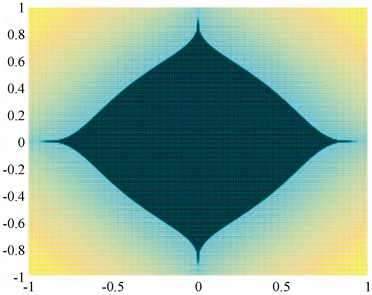
Figure 3. R = 10 norm image
图3. R = 10范数图像

Figure 4. R = 100 norm image
图4. R = 100范数图像
可见通过适当调整 取值在保证产生稀疏解的同时可以增强问题的凸性。由p范数的定义 可知,由于 的非光滑性,导致 是非光滑的,因而我们通过光滑绝对值函数 对 进行光滑逼近。文献 [8] 中对绝对值函数提出如下两个光滑函数:
及 (5)
利用 ,我们得到的模型为:
(6)
其中,
(7)
为叙述方便,令:
(8)
计算函数 的梯度:
(9)
引理1 设D为 中的紧集,若 是D上的光滑函数,则h在D上满足Lipschitz条件,即:
其中 称为Lipschitz常数。
证明:对 ,由 的光滑性及Lagrange中值定理可知:
,其中 位于 之间。
因D为紧集,则 , ,从而 。
引理2设 为紧集, 在D上Lipschitz连续,则 在D上Lipschitz连续。
证明:因D紧且f和g均在D上Lipschitz连续,则 ,满足:
对 ,有:
引理3 若 由(5)定义,则 在紧集D上Lipschitz连续。
证明:对于 的情况,我们有:
当 时,有:
当 时,有:
当 时,有:
当 时,有:
当 或 时,有:
令 ,同理可证存在常数 使得 在紧集D上Lipschitz连续。
最终令 ,我们得到:
引理4 函数 由(7)所定义,则 在紧集D上Lipschitz连续。
证明:计算得:
因 连续可微,且 ,我们有 和 均连续可微。假设集合D有界,则D为紧集,由引理1知 及 在紧集D上Lipschitz连续。
同时由引理3可知 在紧集D上Lipschitz连续,则由引理2可知:
在紧集D上Lipschitz连续,记Lipschitz常数为 ,那么有:
即 在紧集D上Lipschitz连续。
引理5 在紧集D上Lipschitz连续。
证明:计算得 ,由引理1可知 在水平集上光滑,则 在紧集D上Lipschitz连续,记Lipschitz常数为 ,则:
引理6 目标函数梯度 由(9)所定义,则 在紧集D上Lipschitz连续。
证明:计算得 ,则:
3. 基于非精确线搜索的三项共轭梯度法
求问题 的共轭梯度法的具体迭代过程如下:
其中 代表当前迭代点, 代表当前搜索方向, 代表搜索步长, ,不同的 代表不同
的共轭梯度算法。Shouqiang Du和Miao Chen在文献 [9] 中提出了一种新型三项共轭梯度法。具体迭代过程如下:
其中新加入项 可以每步迭代确保目标函数值严格下降,使计算效率更高.本文将利用该共轭梯度法解决信号恢复问题。
算法1 (基于非精确线搜索的共轭梯度法)
步0给出初始参数 ,置 。
步1若满足终止准则 ,停止计算,输出结果 ;否则,转步2。
步2计算搜索方向:
其中,
步3令 ,同时满足:
步4令 ,计算 。
步5令 ,转步1。
假设1令 为常数,假设水平集 是紧集。
定理1 若 是由算法1产生的序列,则:
证明:由文献 [9] 中定理6,本文引理6及假设1可得。
4. 数值实验
本节实验在Intel Core i7-6500U 2.50GHz CPU,8G RAM,Windows10 64位操作系统,MATLAB R2016a环境下进行,所有数值实验结果为测试十次取平均值。
我们对两个不同的绝对值近似函数 和 分别在信号维数n取2048,4096,8192三种情况下,测试随机信号在无噪声和存在噪声干扰时的恢复效果.通过对比信号恢复时间t,相对误差e和迭代步数k来比较范数p和R对算法对信号恢复效果的影响。参数取值如下:A为 的随机高斯矩阵,x为n维随机初始信号, 为初始点, 是一个平均值是0,标准差是0.01的对观测向量b的噪声干扰,p取0.3,0.4,0.5,0.6,R取0,1,10,100 (当R = 0时代表2范数项为0,即目标函数为p范数模型),其他参数取值如下:
1) 我们先对绝对值近似函数 的信号恢复问题进行数值实验,结果如表1至表6所示:

Table 1. Signal dimension n = 2048, no noise interference
表1. 信号维数n = 2048,无噪声干扰
Table 2. Signal dimension n = 2048, Gauss noise interference
表2. 信号维数n = 2048,高斯噪声干扰
Table 3. Signal dimension n = 4096, no noise interference
表3. 信号维数n = 4096,无噪声干扰
Table 4. Signal dimension n = 4096, Gauss noise interference
表4. 信号维数n = 4096,高斯噪声干扰
Table 5. Signal dimension n = 8192, no noise interference
表5. 信号维数n = 8192,无噪声干扰
Table 6. Signal dimension n = 8192, Gauss noise interference
表6. 信号维数n = 8192,高斯噪声干扰
2) 我们再对绝对值近似函数 的信号恢复问题进行数值实验,结果如表7至表12所示:
Table 7. Signal dimension n = 2048, no noise interference
表7. 信号维数n = 2048,无噪声干扰
Table 8. Signal dimension n = 2048, Gauss noise interference
表8. 信号维数n = 2048,高斯噪声干扰
Table 9. Signal dimension n = 4096, no noise interference
表9. 信号维数n = 4096,外界无噪声干扰
Table 10. Signal dimension n = 4096, Gauss noise interference
表10. 信号维数n = 4096,高斯噪声干扰
Table 11. Signal dimension n = 8192, no noise interference
表11. 信号维数n = 8192,无噪声干扰
Table 12. Signal dimension n = 8192, Gauss noise interference
表12. 信号维数n = 8192,高斯噪声干扰
5. 主要结论
通过在不同维度n = 2048,4096,8192下做信号恢复效果分析,我们主要得出以下结论:
1) 相对于p范数模型, 范数模型具有更好的恢复效果,二者在时间和迭代步数相近的情况下, 范数模型对初始信号的精度更高。
2) 做 的值对信号恢复效果影响的横向对比, 的取值对信号恢复的时间和迭代步数影响并不明显;但是 或 时信号的恢复具有更高精度,这是由于当 取值为1~10时2范
数项对p范数的调节使得函数模型的非凸性程度降低,因而提高信号恢复的精度。
3) 做p的值对信号恢复效果影响的纵向对比,显然范数p = 0.6时信号恢复的精度最高,p = 0.3时精度最低。
注:1) 文献 [10] 中提出的模型为
即利用 范数加权从而产生稀疏阶,而本文考虑p范数比1范数更易得到稀疏解,从而利用 范数加权进行信号恢复。
2) 文献 [10] 中的光滑化绝对值函数是文献 [8] 中 。
3) 文献 [11] 中的模型为:
而 较 不易产生稀疏解。取p = 0.3,R = 100对比图形如图5和图6所示:

Figure 5. norm image
图5. 范数图像

Figure 6. norm image
图6. 范数图像
基金项目
内蒙古自然科学基金(2018MS01016)。
文章引用
詹佳明,乌彩英. 求解基于lp+l2范数问题的共轭梯度法
Conjugate Gradient Method for lp+l2 Norm Problems[J]. 应用数学进展, 2019, 08(03): 512-523. https://doi.org/10.12677/AAM.2019.83057
参考文献
- 1. Candes, E.J., Romberg, J. and Tao, T. (2006) Robust Uncertainty Principles: Exact Signal Reconstruction from Highly Incomplete Frequency Information. IEEE Transactions on Information Theory, 52, 489-509. https://doi.org/10.1109/TIT.2005.862083
- 2. Ge, D., Jiang, X. and Ye, Y. (2011) A Note on the Complexity of Lp Minimization. Mathematical Programming, 129, 285-299. https://doi.org/10.1007/s10107-011-0470-2
- 3. Candes, E.J. and Tao, T. (2004) Near Optimal Signal Recovery from Random Projections: Universal Encoding Strategies. IEEE Transactions on Information Theory, 52, 5406-5425. https://doi.org/10.1109/TIT.2006.885507
- 4. Chen, S.S., Donoho, D.L. and Saunders, M.A. (1998) Atomic De-composition by Basis Pursuit. SIAM Journal on Scientific Computing, 20, 33-61. https://doi.org/10.1137/S1064827596304010
- 5. Daubechies, I., Defries, M. and De Mol, C. (2004) An Iterative Thresholding Algorithm for Linear Inverse Problems with a Sparsity Constraint. Communications on Pure and Applied Mathematics, 57, 1413-1457. https://doi.org/10.1002/cpa.20042
- 6. Xu, Z.B., Chang, X., Xu, F., et al. (2012) Regularization: A Thresholding Representation Theory and a Fast Solver. IEEE Transactions on Neural Networks and Learning Systems, 23, 1013-1027. https://doi.org/10.1109/TNNLS.2012.2197412
- 7. Jeevan, K., Pant and Lu, W. (2014) New Improved Algorithms for Compressive Sensing Based on l(p) Norm. Circuits and Systems II: Express Briefs. IEEE Transactions, 61, 198-202.
- 8. Saheya, B., Yu, C.-H. and Chen, J.-S. (2018) Numerical Comparisons Based on Four Smoothing Func-tions for Absolute Value Equation. Journal of Applied Mathematics and Computing, 56, 131-149. https://doi.org/10.1007/s12190-016-1065-0
- 9. Bakhtawar, B., Zabidin, S., Ahmad, A., et al. (2017) A New Modified Three-Term Conjugate Gradient Method with Sufficient Descent Property and Its Global Convergence. Journal of Mathematics, 2017, 1-12.
- 10. Liu, C., Chen, Q., Zhou, B., et al. (2016) L1- and L2-Norm Joint Regularization Based Sparse Signal Reconstruction Scheme. Applied Physics A, 45, 313-323.
- 11. Zhang, Y. and Ye, W.Z. (2017) Sparse Recovery by the Iteratively Reweighted, Algorithm for Elastic, Minimization. Optimization, 66, 1-11. https://doi.org/10.1080/02331934.2017.1359590
NOTES
*通讯作者。