Advances in Applied Mathematics
Vol. 09  No. 09 ( 2020 ), Article ID: 37651 , 15 pages
10.12677/AAM.2020.99176

一类交叉非线性反应扩散方程组的数值模拟

班亭亭,王玉兰

内蒙古工业大学,内蒙古 呼和浩特

收稿日期:2020年8月21日;录用日期:2020年9月10日;发布日期:2020年9月17日

摘要

该文研究一类交叉非线性反应扩散方程组,而交叉扩散项在不稳定时可以创造图灵模式。为了寻找一种简单有效的非线性交叉反应扩散系统的数值方法,本文提出了采用这种新的空间谱插值配点方法模拟了一些数值算例,其结果和理论上的吻合度较好,结果表明了该方法的有效性。

关键词

交叉反应扩散方程,图灵分叉条件,空间谱插值配点方法,数值解

Numerical Simulation of a Class of Cross Nonlinear Reaction-Diffusion Equations

Tingting Ban, Yulan Wang

Inner Mongolia University of Technology, Hohhot Inner Mongolia

Received: Aug. 21st, 2020; accepted: Sep. 10th, 2020; published: Sep. 17th, 2020

ABSTRACT

In this paper, we study a class of cross nonlinear reaction-diffusion equations whose cross diffusion terms can create Turing patterns when they are unstable. In order to find a simple and effective numerical method for nonlinear cross-reaction-diffusion systems, this paper presents a new spatial spectral interpolation method to simulate some numerical examples. The results agree well with the theory, and the results show that the method is effective.

Keywords:Cross Reaction Diffusion Equation, Turing Branching Conditions, Spatial Spectral Interpolation Collocation Method, Numerical Solution

Copyright © 2020 by author(s) and Hans Publishers Inc.

This work is licensed under the Creative Commons Attribution International License (CC BY 4.0).

http://creativecommons.org/licenses/by/4.0/

1. 引言

交叉反应扩散问题在生物学 [1] [2]、医学 [3] [4] [5]、化学 [6] 等中都有广泛的应用,对于求解这类问题的数值方法也有很多,有限元分析法 [7]、无网格方法 [8] 等。在本文中,我们主要研究在理论生物学领域出现的模型,其模型如下:

{ u t = d 11 Δ u + d 12 Δ v + f ( u , v ) v t = d 21 Δ u + d 22 Δ v + g ( u , v ) (1)

其中: u ( x , y , t ) v ( x , y , t ) 是未知函数, d 11 , d 12 , d 21 , d 22 是扩散系数, Δ = 2 / x 2 + 2 / y 2 是拉普拉斯算子, ( x , y ) Ω t > 0 是在光滑的边界 Ω 上的齐次Neumann边界条件,即 u / n = v / n = 0 f ( u , v ) , g ( u , v ) 是已知的光滑函数。

本文考虑了交叉反应扩散系统的以下两组非线性情况:

1) f ( u , v ) = u ( α β u ) c u v m v + 1 , g ( u , v ) = s u v m v + 1 r v

2) f ( u , v ) = u ( σ ( 1 u β ) ( 1 + α v ) v ) , g ( u , v ) = v ( ( 1 + α v ) u 1 )

2. 空间谱插值配点方法的描述

在本文中,我们使用空间谱插值配点方法来解决模型(1)。

从参考文献 [9] [10] 中,我们可以得到离散序列 u 1 , u 2 , , u N 的插值函数 I N u ( x ) 可以写成:

u ( x ) ~ I N u ( x ) = m = 1 N u m S N ( x x m ) (2)

其中 S N ( x ) = sin ( π x / h ) ( 2 π / h ) tan ( x / 2 ) I N 对于任何函数,都是这样的插值算子, u ( x ) 在区间 [ 0 , 2 π ] 定义为 u j = u ( j h ) , j = 1 , , N , x j x m = ( j m ) h ,插值空间为 s p a n { S N ( x j h ) , j = 1 , 2 , , N } 。由此推导出n阶导数的简单表达式并不难 I N u ( x ) x j = j h 处的n阶导数的简单表达式并不难,为:

I N u ( n ) ( x j ) = m = 1 N u m S N ( n ) ( x j x m ) (3)

其中 D N ( n ) = [ S N ( n ) ( x j x m ) ] i , j = 1 , 2 , , N 被称为第n个谱微分矩阵 [9]。

这里我们考虑有限空间域 Ω = [ 0 , 2 π ] × [ 0 , 2 π ] 。我们定义 N 2 个等间距的网格点在区域 Ω 上,因此

( x i , y j ) = ( i h , j h ) , i , j = 1 , 2 , 3 , , N .

其中 h = 2 π N 对于给定的有限自然数 N 。使用(2)则配点函数 I N u ( x , y , t ) I N v ( x , y , t ) 关于函数 u ( x , y , t ) v ( x , y , t ) 可以被写为:

u ( x , y , t ) ~ I N u ( x , y , t ) = i = 1 N j = 1 N S N ( x x i ) S N ( y y i ) u ( x i , y j , t ) v ( x , y , t ) ~ I N v ( x , y , t ) = i = 1 N j = 1 N S N ( x x i ) S N ( y y i ) v ( x i , y j , t ) (4)

其中 u i , j = u ( x i , y j , t ) , v i , j = v ( x i , y j , t ) , i , j = 1 , 2 , , N 。因此,下列关系在搭配点 ( x p , y q ) 处成立:

u ( x p , y q , t ) ~ I N u ( x p , y q , t ) = i = 1 N j = 1 N S N ( x p x i ) S N ( y q y i ) u ( x i , y j , t ) v ( x p , y q , t ) ~ I N v ( x p , y q , t ) = i = 1 N j = 1 N S N ( x p x i ) S N ( y q y i ) v ( x i , y j , t ) (5)

u ( 2 , 0 ) ( x p , y q , t ) ~ I N u ( 2 , 0 ) ( x p , y q , t ) = 2 u ( x p , y q , t ) x 2 = i = 1 N j = 1 N S N ( 2 ) ( x p x i ) S N ( y q y i ) u ( x i , y j , t ) u ( 0 , 2 ) ( x p , y q , t ) ~ I N u ( 0 , 2 ) ( x p , y q , t ) = 2 u ( x p , y q , t ) y 2 = i = 1 N j = 1 N S N ( x p x i ) S N ( 2 ) ( y q y i ) u ( x i , y j , t ) v ( 2 , 0 ) ( x p , y q , t ) ~ I N v ( 2 , 0 ) ( x p , y q , t ) = 2 v ( x p , y q , t ) x 2 = i = 1 N j = 1 N S N ( 2 ) ( x p x i ) S N ( y q y i ) v ( x i , y j , t ) v ( 0 , 2 ) ( x p , y q , t ) ~ I N v ( 0 , 2 ) ( x p , y q , t ) = 2 v ( x p , y q , t ) y 2 = i = 1 N j = 1 N S N ( x p x i ) S N ( 2 ) ( y q y i ) v ( x i , y j , t )

注意的是

u = [ u 11 , u 21 , , u N 1 , u 12 , u 22 , , u N 2 , u 1 N , , u N N ] T , v = [ v 11 , v 21 , , v N 1 , v 12 , v 22 , , v N 2 , v 1 N , , v N N ] T , (6)

因此,公式(5)可以被写成一下矩阵形式:

u ( 2 , 0 ) = D N ( 2 , 0 ) u , u ( 0 , 2 ) = D N ( 0 , 2 ) u , v ( 2 , 0 ) = D N ( 2 , 0 ) v , v ( 0 , 2 ) = D N ( 0 , 2 ) v . (7)

D N ( 2 , 0 ) u = D N ( 2 ) E N , D N ( 0 , 2 ) = E N D N ( 2 ) , D N ( 0 , 0 ) = E N E N ,

其中 E N 是N阶单位矩阵, 是矩阵的克罗内克积,相反地。二阶谱微分矩阵为:

D N ( 2 ) = ( π 2 3 h 2 1 6 1 2 csc 2 ( 1 h 2 ) 1 2 csc 2 ( 1 h 2 ) 1 2 csc 2 ( 2 h 2 ) 1 2 csc 2 ( 2 h 2 ) 1 2 csc 2 ( 2 h 2 ) 1 2 csc 2 ( 1 h 2 ) 1 2 csc 2 ( 3 h 2 ) π 2 3 h 2 1 6 1 2 csc 2 ( 3 h 2 ) 1 2 csc 2 ( 1 h 2 ) 1 2 csc 2 ( 2 h 2 ) 1 2 csc 2 ( 2 h 2 ) 1 2 csc 2 ( 1 h 2 ) 1 2 csc 2 ( 1 h 2 ) 1 2 csc 2 ( 1 h 2 ) π 2 3 h 2 1 6 ) (8)

结合等式(6)和等式(7),Equation (1)可以写成以下系统:

t [ u v ] = [ d 11 D d 12 D d 21 D d 22 D ] [ u v ] = [ f ( u , v ) g ( u , v ) ] (9)

这里

[ u , v ] = [ u 11 , , u N 1 , u 12 , , u N 2 , u 1 N , , u N N , v 11 , , v N 1 , v 12 , , v N 2 , v 1 N , , v N N ] ,

D = D N ( 2 , 0 ) + D N ( 0 , 2 ) = D N ( 2 ) E N + E N D N ( 2 ) ,

[ f ( u , v ) , g ( u , v ) ] = [ f ( u 11 , v 11 ) , , f ( u N N , v N N ) , g ( u 11 , v 11 ) , , g ( u N N , v N N ) ]

利用Matlab中的ode45求解器求解系统(9),得到系统(1)的数值解。

3. 系统分叉分析

在这一部分,我们给出了交叉反应扩散问题的图灵分叉分析。我们假设非扩散系统(1)的平衡点是 E * = ( u 0 , v 0 ) ,所以

{ f ( u 0 , v 0 ) = 0 g ( u 0 , v 0 ) = 0 (10)

现在我们对平衡点 E * 进行线性稳定性分析。我们在E处对系统的雅可比矩阵 A 0 进行

A 0 = [ f u ( u 0 , v 0 ) f v ( u 0 , v 0 ) g u ( u 0 , v 0 ) g v ( u 0 , v 0 ) ] (11)

A 0 的特征根由

λ 1 , 2 ( 0 ) = 1 2 [ t r ( A 0 ) ± [ t r ( A 0 ) ] 2 4 det ( A 0 ) ]

其中 t r ( A 0 ) = f u ( u 0 , v 0 ) + g v ( u 0 , v 0 ) det ( A 0 ) = [ f u ( u 0 , v 0 ) ] × [ g v ( u 0 , v 0 ) ] [ g u ( u 0 , v 0 ) ] × [ f v ( u 0 , v 0 ) ]

一般情况下,如果特征值的实部 λ 1 , 2 ( 0 ) 为负值,则非扩散系统(1)是稳定的。

接下来,我们导出了交叉扩散驱动的不稳定性条件,并证明了这些是在没有交叉扩散的情况下经典扩散驱动不稳定性条件的推广。

A k = [ b 11 b 12 b 21 b 22 ] k 2 [ d 11 d 12 d 21 d 22 ] (12)

其中 b 11 = f u ( u 0 , v 0 ) , b 12 = f v ( u 0 , v 0 ) , b 21 = g u ( u 0 , v 0 ) , b 22 = g v ( u 0 , v 0 )

特征根由 A k 给出:

λ 1 , 2 ( k ) = 1 2 [ t r ( A k ) ± [ t r ( A k ) ] 2 4 det ( A k ) ]

其中 t r ( A k ) = b 11 + b 22 k 2 ( d 11 + d 22 ) det ( A k ) = ( d 11 d 22 d 12 d 21 ) k 4 ( b 11 d 22 + b 22 d 11 b 12 d 21 b 21 d 12 ) k 2 + ( b 11 b 22 b 12 b 21 )

图灵分岔发生在没有非扩散时稳定的等分态,但在交叉扩散时变得不稳定。因此, E * 成为交叉扩散系统(1)不稳定点的唯一途径是特征值 λ 1 , 2 ( k ) 的实部是正的,那么交叉扩散系统(1)是不稳定的。

4. 数值实验

在这一部分中,我们给出了一些数值插图,以更好地解释上述分析结果使用不同的初始条件和参数。如果非线性项为 f ( u , v ) = u ( α β u ) c u v m v + 1 , g ( u , v ) = s u v m v + 1 r v 时,则反应扩散体系(1)则变为例1 [10] 形式。其中 [10] E * = ( u 0 , v 0 ) u 0 = s ( m α c ) + s 2 ( m α c ) 2 + 4 c m r s β 2 m s β

v 0 = s u 0 r m r . A 0 =[ β u 0 c u 0 ( m v 0 +1 ) 2 s v 0 ( m v 0 +1 ) ms u 0 v 0 ( m v 0 +1 ) 2 ] .

例1 考虑以下形式的交叉反应扩散模型 [10]:

{ u t d 11 Δ u d 12 Δ v = u ( α β u ) c u v m v + 1 , ( x , t ) Ω × [ 0 , ] v t d 21 Δ u d 22 Δ v = s u v m v + 1 r v , ( x , t ) Ω × [ 0 , ] u n = v n = 0 , ( x , t ) Ω × [ 0 , ] u ( x , 0 ) = u 0 ( x ) 0 , v ( x , 0 ) = v 0 ( x ) 0 , x Ω (13)

这里 d 11 , d 12 , d 21 , d 22 > 0 α , β , γ , s , m , c 为常数, t R + 为时间变量, x , y R 是空间变量, u , v 是t与 x , y 的函数。其中参数1 β = 1 , c = 1 , γ = 1 , s = 1 , m = 4 , α = 0.8 , d 11 = 1 , d 22 = 10 , d 12 = 1 , d 21 = 10 和参数2 β = 1 , c = 1 , γ = 2 , s = 1 , m = 4 , α = 1.2 , d 11 = 1 , d 22 = 1 , d 12 = 0.4 , d 21 = 2 ,固定一个初始条件 v = 0.5 o n e s ( N ) ,当u以及参数变化时模拟的结果见图1~11,具体初始条件见表1

如果非线性项为 f ( u , v ) = u ( σ ( 1 u β ) ( 1 + α v ) v ) , g ( u , v ) = v ( ( 1 + α v ) 1 ) 时,则反应扩散体系(1)则变成例2形式。其中 [11] u 0 = β ( 1 v 0 ( 1 + α v 0 ) σ ) ,而 v 0 是下列三次多项式方程 β α 2 v 3 + 2 β α v 2 + β ( 1 α σ ) v + σ ( 1 β ) = 0 的根。 A 0 = [ a 11 a 12 a 21 a 22 ] a 11 = σ 2 σ u 0 β v 0 α v 0 2 a 12 = u 0 2 α u 0 v 0 a 21 = v 0 + α v 0 2 a 22 = u 0 + 2 α u 0 v 0 1

例2 考虑以下形式的交叉反应扩散模型[11]:

{ u t d 11 Δ u d 12 Δ v = u ( σ ( 1 u β ) ( 1 + α v ) v ) , ( x , t ) Ω × [ 0 , ] v t d 21 Δ u d 22 Δ v = v ( ( 1 + α v ) u 1 ) , ( x , t ) Ω × [ 0 , ] u n = v n = 0 , ( x , t ) Ω × [ 0 , ] u ( x , 0 ) = u 0 ( x ) 0 , v ( x , 0 ) = v 0 ( x ) 0 , x Ω (14)

这里 d 11 , d 12 , d 21 , d 22 > 0 α , β , σ 为常数, t R + 为时间变量, x , y R 是空间变量, u , v 是t与 x , y 的函数。其中 δ = 4 , α = 0.3 , β = 1.5 , d 11 = 0.5 , d 22 = 10 ,参数1为 d 12 = 0.2 , d 21 = 10.5 ;参数2为 d 12 = 1 , d 21 = 0.2 ,固定一个初始条件 v = 0.5 o n e s ( N ) ,当v固定时改变参数和u得到的模拟结果见图12~19,固定 u = cos ( x 2 + y 2 ) 时得到的模拟结果见图20图21,具体的初始条件见表2

Table 1. The different initial conditions corresponding to the numerical solution and pattern in example 1 are shown in Figures 1~11

表1. 例1中数值解和斑图所对应的不同的初始条件在图1~11

Figure 1. Shows the numerical solution of u = o n e s ( N ) + sech ( x 2 / 0.02 9 + 2 y / 0.01 ) in parameter 1 and initial condition of example 1

图1. 在参数1和初始条件为 u = o n e s ( N ) + sech ( x 2 / 0.02 9 + 2 y / 0.01 ) 的数值解

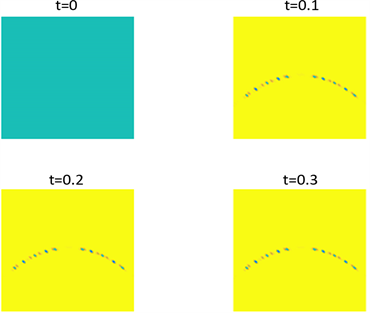
Figure 2. Shows the pattern of u = o n e s ( N ) + sech ( x 2 / 0.02 9 + 2 y / 0.01 ) in parameter 1 and initial condition of example 1

图2. 例1在参数1和初始条件为 u = o n e s ( N ) + sech ( x 2 / 0.02 9 + 2 y / 0.01 ) 的斑图

Figure 3. Shows the pattern of u = o n e s ( N ) + sech ( x 2 / 0.02 9 + 2 y / 0.01 ) in parameter 2 and initial condition of example 1

图3. 例1在参数2和初始条件为 u = o n e s ( N ) + sech ( x 2 / 0.02 9 + 2 y / 0.01 ) 的斑图

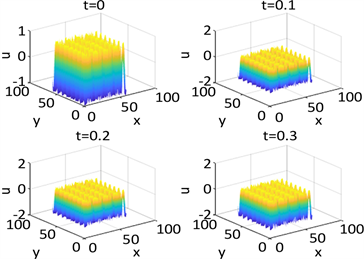
Figure 4. Shows the numerical solution of u = sin ( x 2 / 0.02 9 + 2 y / 0.01 ) in parameter 1 and initial condition of example 1

图4. 例1在参数1和初始条件为 u = sin ( x 2 / 0.02 9 + 2 y / 0.01 ) 的数值解

Figure 5. Shows the pattern of u = sin ( x 2 / 0.02 9 + 2 y / 0.01 ) in parameter 1 and initial condition of example 1

图5. 例1在参数1和初始条件为 u = sin ( x 2 / 0.02 9 + 2 y / 0.01 ) 的斑图

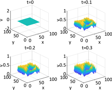
Figure 6. Shows the numerical solution of u = sin ( exp ( ( x 0.4 ) 2 + ( y + 0.4 ) 2 ) ) sin ( cos ( ( x + 0.4 ) 3 + ( y 0.4 ) 2 ) ) in parameter 1 and initial condition of example 1

图6. 例1在参数1和初始条件为 u = sin ( exp ( ( x 0.4 ) 2 + ( y + 0.4 ) 2 ) ) sin ( cos ( ( x + 0.4 ) 3 + ( y 0.4 ) 2 ) ) 的数值解

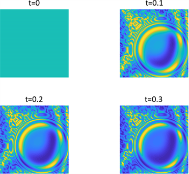
Figure 7. Shows the pattern of u = sin ( exp ( ( x 0.4 ) 2 + ( y + 0.4 ) 2 ) ) sin ( cos ( ( x + 0.4 ) 3 + ( y 0.4 ) 2 ) ) in parameter 1 and initial condition of example 1

图7. 例1在参数1和初始条件为 u = sin ( exp ( ( x 0.4 ) 2 + ( y + 0.4 ) 2 ) ) sin ( cos ( ( x + 0.4 ) 3 + ( y 0.4 ) 2 ) ) 的斑图

Figure 8. Shows the numerical solution of u = sech ( ( x 3 y 5 ) 3 ) in parameter 1 and initial condition of example 1

图8. 例1在参数1和初始条件为 u = sech ( ( x 3 y 5 ) 3 ) 的数值解

Figure 9. Shows the pattern of u = sech ( ( x 3 y 5 ) 3 ) in parameter 1 and initial condition of example 1

图9. 例1在参数1和初始条件为 u = sech ( ( x 3 y 5 ) 3 ) 的斑图

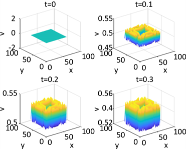
Figure 10. Shows the numerical solution of u = cos ( sin ( x 3 + y 5 ) ) in parameter 1 and initial condition of example 1

图10. 例1在参数1和初始条件为 u = cos ( sin ( x 3 + y 5 ) ) 的数值解

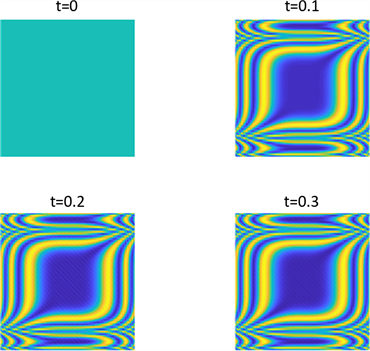
Figure 11. Shows the pattern of u = cos ( sin ( x 3 + y 5 ) ) in parameter 1 and initial condition of example 1

图11. 图为例1在参数1和初始条件为 u = cos ( sin ( x 3 + y 5 ) ) 的斑图

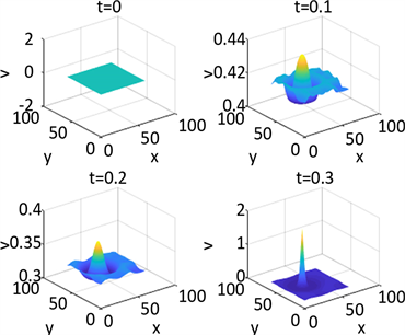
Figure 12. Shows the numerical solution of u = sin ( sin ( ( x 0.4 ) 3 ( y + 0.4 ) 2 ) ) cos ( exp ( ( x + 0.4 ) 2 + ( y 0.4 ) 2 ) ) in parameter 1 and initial condition of example 2

图12. 为例2在参数1和初始条件为 u = sin ( sin ( ( x 0.4 ) 3 ( y + 0.4 ) 2 ) ) cos ( exp ( ( x + 0.4 ) 2 + ( y 0.4 ) 2 ) ) 的数值解

Figure 13. Shows the pattern of u = sin ( sin ( ( x 0.4 ) 3 ( y + 0.4 ) 2 ) ) cos ( exp ( ( x + 0.4 ) 2 + ( y 0.4 ) 2 ) ) in parameter 1 and initial condition of example 2

图13. 为例2在参数1和初始条件为 u = sin ( sin ( ( x 0.4 ) 3 ( y + 0.4 ) 2 ) ) cos ( exp ( ( x + 0.4 ) 2 + ( y 0.4 ) 2 ) ) 的斑图

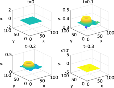
Figure 14. Shows the numerical solution of u = sin ( sin ( ( x 0.4 ) 3 ( y + 0.4 ) 2 ) ) + cos ( exp ( ( x + 0.4 ) 2 + ( y 0.4 ) 2 ) ) in parameter 2 and initial condition of example 2

图14. 图为例2在参数2和初始条件为 u = sin ( sin ( ( x 0.4 ) 3 ( y + 0.4 ) 2 ) ) + cos ( exp ( ( x + 0.4 ) 2 + ( y 0.4 ) 2 ) ) 的数值解

Figure 15. Shows the pattern of u = sin ( sin ( ( x 0.4 ) 3 ( y + 0.4 ) 2 ) ) + cos ( exp ( ( x + 0.4 ) 2 + ( y 0.4 ) 2 ) ) in parameter 2 and initial condition of example 2

图15. 为例2在参数2和初始条件为 u = sin ( sin ( ( x 0.4 ) 3 ( y + 0.4 ) 2 ) ) + cos ( exp ( ( x + 0.4 ) 2 + ( y 0.4 ) 2 ) ) 的斑图

Figure 16. Shows the numerical solution of u = sech ( π ( x 2 + y 2 ) ) in parameter 1 and initial condition of example 2

图16. 图为例2在参数1和初始条件为 u = sech ( π ( x 2 + y 2 ) ) 的数值解

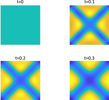
Figure 17. Shows the pattern of u = sech ( π ( x 2 + y 2 ) ) in parameter 1 and initial condition of example 2

图17. 为例2在参数1和初始条件为 u = sech ( π ( x 2 + y 2 ) ) 的斑图

Figure 18. Shows the numerical solution with the initial condition of u = cos ( exp ( sin ( x 2 y 2 ) ) ) example 2

图18. 图为例2在参数1和初始条件为 u = cos ( exp ( sin ( x 2 y 2 ) ) ) 的数值解

Figure 19. Shows the pattern of u = cos ( exp ( sin ( x 2 y 2 ) ) ) in parameter 1 and initial condition of example 2

图19. 为例2在参数1和初始条件为 u = cos ( exp ( sin ( x 2 y 2 ) ) ) 的斑图

Figure 20. Shows the numerical solution of u = cos ( x 2 + y 2 ) , v = sin ( x 2 / 0.02 9 + 2 y / 0.01 ) in parameter 2 and initial condition of example 2

图20. 图为例2在参数2和初始条件为 u = cos ( x 2 + y 2 ) , v = sin ( x 2 / 0.02 9 + 2 y / 0.01 ) 的数值解

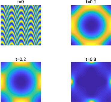
Figure 21. Shows the pattern of u = cos ( x 2 + y 2 ) , v = sin ( x 2 / 0.02 9 + 2 y / 0.01 ) in parameter 2 and initial condition of example 2

图21. 为例2在参数2和初始条件为 u = cos ( x 2 + y 2 ) , v = sin ( x 2 / 0.02 9 + 2 y / 0.01 ) 的斑图

Table 2. The different initial conditions corresponding to the numerical solution and pattern in example 2 are shown in Figures 12~21

表2. 例2中数值解和斑图所对应的不同的初始条件在图12~21

5. 结论

本文用谱插值配点方法求解一类非线性交叉反应扩散模型,数值结果表明了该方法与理论吻合较好。本文所有程序由matlab2017b算得。

致谢

感谢王玉兰老师的支持与帮助。

文章引用

班亭亭,王玉兰. 一类交叉非线性反应扩散方程组的数值模拟
Numerical Simulation of a Class of Cross Nonlinear Reaction-Diffusion Equations[J]. 应用数学进展, 2020, 09(09): 1493-1507. https://doi.org/10.12677/AAM.2020.99176

参考文献

  1. 1. 戴婉仪, 付一平. 一类具有交叉扩散捕食者-食饵系统的时间周期解的存在性与稳定性[J]. 应用数学学报, 2007, 30(3): 385-394.

  2. 2. 张晓晶. 带交叉扩散的捕食-食饵模型的研究[D]: [硕士学位论文]. 西安: 西安工程大学, 2015.

  3. 3. Tyson, J.J. (1976) The Belousov-Zhabotinskii Reaction. Lecture Notes in Biomathematics 10. Springer-Verlag, Heidelberg. https://doi.org/10.1007/978-3-642-93046-1

  4. 4. 陶纪元. 一类具有交叉感染的流行病模型的数学分析[D]: [硕士学位论文]. 北京: 北京理工大学, 1996.

  5. 5. 李正元, 陶纪元, 叶其孝. 具交叉感染的流行病模型的数学分析[J]. 高校应用数学学报B辑, 2016, 14(4): 389-400.

  6. 6. 卢创业. 血管肿瘤生长模型的定性分析[D]: [硕士学位论文]. 广州: 广东工业大学, 2016.

  7. 7. 杨水龙. 一个化学反应扩散方程奇异行波摄动解[C]//数学·力学·物理学·高新技术研究进展——2002(9)卷——中国数学力学物理学高新技术交叉研究会第9届学术研讨会论文集, 2002.

  8. 8. 江成顺, 崔霞. 一类非线性反应扩散方程组的有限元分析[J]. 计算数学, 2000, 22(1):103-112.

  9. 9. 闭海, 鲁统超. 一类非线性反应扩散方程的配置方法[J]. 山东大学学报(理学版), 2004, 39(2): 41-46, 55.

  10. 10. Zhang, X. (2015) Efficient Solution of Differential Equation Based on MATLAB: Spectral Method Principle and Implementation. Mechanical Industry Press, Beijing.

  11. 11. Yao, S.-W., Ma, Z.-P. and Yue, J.-L. (2018) Bistability and Turing Pattern Induced by Cross Fraction Diffusion in a Predator-Prey Model. Physica A Statistical Mechanics & Its Applications, 509, 982-988. https://doi.org/10.1016/j.physa.2018.06.072

期刊菜单