Pure Mathematics
Vol.
11
No.
04
(
2021
), Article ID:
41776
,
8
pages
10.12677/PM.2021.114071
基于梯度方法的线性多延时系统参数辩识
徐文瀚
上海大学理学院,上海

收稿日期:2021年3月13日;录用日期:2021年4月15日;发布日期:2021年4月22日

摘要
针对一类线性多延时系统,提出一种基于梯度和最小二乘方法的参数辨识算法。该算法首先将系数矩阵和延时量的联合估计问题转化为仅关于延时量的优化问题,然后基于动量梯度法求出延时量的估计值,最后利用矩阵方程的最小二乘解得出系数矩阵的估计值,仿真结果表明,该算法有较好的辨识效果。
关键词
线性多延时系统,动量梯度法,最小二乘方法
Parameter Identification of Linear Multi-Delay System Based on Gradient Method
Wenhan Xu
School of Science, Shanghai University, Shanghai

Received: Mar. 13th, 2021; accepted: Apr. 15th, 2021; published: Apr. 22nd, 2021

ABSTRACT
For a class of linear systems with multiple delays, a new parameter identification algorithm based on gradient and least square method is proposed. Firstly, the joint estimation problem of coefficient matrix and time delay is transformed into the optimization problem which only estimates time delay. Then, the estimated value of time delay is obtained based on momentum gradient method. Finally, by using the least square solution of matrix equation, the estimated value of coefficient matrix is obtained. The algorithm has good identification effect.
Keywords:Linear Multi-Delay System, Momentum Gradient Method, Least Square Method

Copyright © 2021 by author(s) and Hans Publishers Inc.
This work is licensed under the Creative Commons Attribution International License (CC BY 4.0).
http://creativecommons.org/licenses/by/4.0/


1. 引言
随着社会的发展和科技的进步,延时系统在生物、经济和自动化控制等诸多领域日益受到重视 [1] [2]。参数辨识是设计、分析与控制实际系统的重要前提 [3]。
时域方法 [4] [5] [6] 是延时系统参数辨识领域的重要方法。基于梯度的辨识算法近年来受到许多学者的关注。文献 [7] [8] [9] 应用变分方法计算梯度并提出一种参数辨识算法;文献 [10] 求得了准则函数对参数的梯度所满足的系统,并由此给出了一种辨识算法。
本文受文献 [11] 启发,研究了一类线性多延时系统的系数和延时量的辨识问题。本文的主要工作是设计了关于系数矩阵和延时量的准则函数,利用最小二乘原理给出了固定延时量时系数矩阵的最小二乘解,从而将系数矩阵和延时量的同时估计问题看作仅关于延时量的估计问题,利用梯度方法求解优化问题得出延时量,最终用估计出的延时量求解矩阵方程求得系数矩阵。
2. 问题描述
考虑以下线性延时系统:
(1)
其中 表示状态向量; 表示控制向量; , 是系统的参数矩阵;初始函数 ;这里假定系统的延时量满足 。
记 ,。
定义2.1 设矩阵 ,称 为Q的Frobenius范数。
命题2.1 设 ,则
引理2.1 [12] 若A是列满秩矩阵,B是行满秩矩阵,矩阵 满足
那么在最小二乘意义下上式有唯一解 。
命题2.2 设矩阵函数 可逆且可导,则 。
命题2.3 设矩阵函数 可导,则
本文的目的是通过求解如下的优化问题辨识参数 ,
(2)
其中
(3)
3. 算法的推导
固定延时量 ,式(2)中 有唯一最小二乘解。从而对优化问题(2)的求解可转化为只与 有关的优化问题。接下来,利用新目标函数关于 的梯度采用动量梯度法估计延时量。最后,求系数矩阵关于式(2)的最小二乘解。
3.1. 梯度的计算
定理3.1 对于式(2)所述的优化问题,当 固定时有唯一最小二乘解
(4)
其中
(5)
(6)
证明。
由命题2.1,上式可写为 。
由引理2.1上式中 有唯一最小二乘解。
(7)
根据定理3.1可知,优化问题(2)可以转化为
(8)
接下来分三个定理求 。
定理3.2 设 ,则
证明。
定理3.3 设 ,则
其中 。
证明。
由命题2.2得
定理3.4 式(8)对延时量 的偏导数如下
(9)
证明。
3.2. 算法描述
本文采用动量梯度法进行联合估计(见算法1)。
4. 数值算例
本节给出两个数值算例来验证结果的有效性
例4.1 考虑不稳定的线性单延时系统(1),系统参数如下
输入函数为 ,初始函数为 。
初始点 ,参数 。
利用算法1出参数
用算法1估计例4.1中延时量的迭代过程如图1所示。

Figure 1. Iterative process of delay estimation
图1. 延时量估计的迭代过程
例4.2 考虑线性多延时系统(1),系统参数如下
输入函数为 ,初始函数为 .
初始点 ,参数 .
利用算法1出参数
用算法1估计例4.2中两个延时量的迭代过程通过等高线图方式呈现如图2所示。将图2中目标函数和迭代过程用三维曲面呈现后如图3所示。

Figure 2. Iterative process of two delay estimation
图2. 两个延时量估计的迭代过程
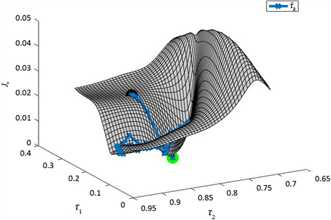
Figure 3. The iterative process and objective function of the delay amount
图3. 延时量的迭代过程及目标函数
5. 结论
针对线性多延时系统,给出了一种含积分的目标函数。通过最小二乘方法将联合参数的目标函数转化为仅依赖延时量的非线性函数。采用动量梯度方法求解关于延时量的优化问题。确定延时量后求矩阵方程的最小二乘解估计系数矩阵。通过数值仿真验证了算法的有效性。
文章引用
徐文瀚. 基于梯度方法的线性多延时系统参数辩识
Parameter Identification of Linear Multi-Delay System Based on Gradient Method[J]. 理论数学, 2021, 11(04): 578-585. https://doi.org/10.12677/PM.2021.114071
参考文献
- 1. Kim, A.V. and Ivanov, A.V. (2015) Systems with Delays: Analysis, Control, and Computations. John Wiley & Sons, Hoboken. https://doi.org/10.1002/9781119117841
- 2. Hale, J.K. and Verduyn Lunel, S.M. (1993) Introduction to Functional Differential Equations. Springer Science & Business Media, Berlin, Volume 99. https://doi.org/10.1007/978-1-4612-4342-7
- 3. Isermann, R. and Münchhof, M. (2011) Identification of Dynamic Systems: An Introduction with Application. Springer Publishing Company, Incorporated, Berlin. https://doi.org/10.1007/978-3-540-78879-9_1
- 4. Bedoui, S., Ltaief, M. and Abderrahim, K. (2012) New Results on Discrete Time Delay Systems Identification. International Journal of Automation and Computing, 9, 570-577. https://doi.org/10.1007/s11633-012-0681-x
- 5. Sassi, A., Bedoui, S. and Abderrahim, K. (2013) Time Delay System Identification Based on Optimization Approaches. 2013 17th International Conference on System Theory, Control and Computing (ICSTCC), Sinaia, 11-13 October 2013, 473-478. https://doi.org/10.1109/ICSTCC.2013.6689003
- 6. Orlov, Y., Belkoura, L., Richard, J.P., et al. (2003) Adaptive Identification of Linear Time-Delay Systems. International Journal of Robust and Nonlinear Control, 13, 857-872. https://doi.org/10.1002/rnc.850
- 7. Lin, Q., Loxton, R., Xu, C., et al. (2015) Parameter Estimation for Nonlinear Time-Delay Systems with Noisy Output Measurements. Automatica, 60, 48-56. https://doi.org/10.1016/j.automatica.2015.06.028
- 8. Loxton, R., Teo, K.L. and Rehbock, V. (2010) An Optimi-zation Approach to State-Delay Identification. IEEE Transactions on Automatic Control, 55, 2113-2119. https://doi.org/10.1109/TAC.2010.2050710
- 9. Michalska, H. and Lu, M. (2006) Delay Identification in Linear Differential Difference Systems. Proceedings of the 8th WSEAS International Conference on Automatic Control, Mod-eling & Simulation, San Diego, 13-15 December 2006, 297-304. https://doi.org/10.1109/CDC.2006.377540
- 10. Ren, X., Rad, A.B., Chan, P., et al. (2005) Online Identification of Continuous Time Systems with Unknown Time Delay. IEEE Transactions on Automatic Control, 50, 1418-1422. https://doi.org/10.1109/TAC.2005.854640
- 11. Ghoul, Y., Taarit, K.I. and Ksouri, M. (2016) Separable Identifi-cation of Continuous-Time Systems Having Multiple Unknown Time Delays from Sampled Data. 2016 4th International Conference on Control Engineering & Information Technology (CEIT), Hammamet, 16-18 December 2016, 1-6. https://doi.org/10.1109/CEIT.2016.7929051
- 12. Ding, F., Liu, P.X. and Ding, J. (2008) Iterative Solutions of the Generalized Sylvester Matrix Equations by Using the Hierarchical Identification Principle. Applied Mathematics and Computation, 197, 41-50. https://doi.org/10.1016/j.amc.2007.07.040