Advances in Applied Mathematics
Vol.
12
No.
10
(
2023
), Article ID:
73737
,
12
pages
10.12677/AAM.2023.1210422
abcd Boussinesq系统的高阶中心间断 Galerkin-有限元方法
夏有伟,程用平*
重庆交通大学数学与统计学院,重庆
收稿日期:2023年9月13日;录用日期:2023年10月8日;发布日期:2023年10月16日

摘要
Boussinesq类型的方程是一类重要的非线性色散浅水波方程,广泛应用于研究小振幅浅水波的传播现象。我们考虑一个含有四个参数的Boussinesq系统:abcd Boussinesq系统,并针对该系统设计了一个高阶中心间断Galerkin-有限元方法。该方法首先将abcd Boussinesq系统改写为守恒律方程与椭圆型方程的一个耦合系统,然后采用中心局部间断Galerkin方法求解守恒律方程,使用有限元方法求解椭圆型方程,最后我们通过一系列的数值算例验证所提出方法的高阶精度和有效性。
关键词
非线性浅水波方程,Boussinesq系统,中心间断Galerkin方法,有限元方法

High Order Central Discontinuous Galerkin-Finite Element Methods for the abcd Boussinesq System
Youwei Xia, Yongping Cheng*
College of Mathematics and Statistics, Chongqing Jiaotong University, Chongqing
Received: Sep. 13th, 2023; accepted: Oct. 8th, 2023; published: Oct. 16th, 2023

ABSTRACT
Boussinesq type equations are an important class of nonlinear dispersive shallow water wave equations, it has been widely studied to model the propagation phenomena of small amplitude shallow water waves. In this work, we consider a Boussinesq system with four parameters: abcd Boussinesq system, and design a high order central discontinuous Galerkin-finite element methods for solving this system. In our numerical approach, we first reformulate the abcd Boussinesq system into a coupled system of conservation law and elliptic equations. Then we propose a family of high order numerical methods which discretize the conservation law with central local discontinuous Galerkin methods and the elliptic equations with continuous finite element methods. Different types of numerical tests are provided to illustrate the accuracy and effectiveness of the proposed schemes.
Keywords:Nonlinear Shallow Water Equations, Boussinesq System, Central Discontinuous Galerkin Methods, Finite Element Methods

Copyright © 2023 by author(s) and Hans Publishers Inc.
This work is licensed under the Creative Commons Attribution International License (CC BY 4.0).
http://creativecommons.org/licenses/by/4.0/


1. 引言
Boussinesq方程是一类重要的非线性偏微分方程,它是模拟近海岸浅水波传播现象的重要工具之一。关于水波的Boussinesq近似,最初是由Boussinesq [1] 在1871年提出,从欧拉方程出发推导出了第一个Boussinesq方程。此后,不同类型的Boussinesq方程相继被提出,例如“good” Boussinesq方程 [2] 与improved Boussinesq方程 [3] 。直到2002年,Bona等人 [4] 提出了一个更一般化的Boussinesq方程,即abcd Boussinesq系统:
(1)
这里, 表示水的自由表面与其静止位置的垂直偏差,u表示水平方向上的速度,a,b,c,d是四个常数,满足以下的关系式:
, , 。 (2)
四个参数a,b,c,d的不同取值对应着不同的浅水波模型。例如,当 时方程(1)对应着经典的Boussinesq方程, 时相应地变成了耦合的Benjamin-Bona-Mahony (BBM)方程, 时也就是耦合的Korteweg-de Vries (KdV)方程。
目前关于Boussinesq类型方程的数值方法已经得到了很好的发展。例如Peregrine等人 [5] 在1966年针对经典的Boussinesq方程提出了一个有限差分近似方法。Bona等人 [6] 在2007年采用带有周期光滑样条基函数的Galerkin方法数值求解了耦合的KdV-KdV系统。2019年,Burtea和Courtès [7] 关于abcd Boussinesq系统提出了一个完全离散的有限体积方法,并证明了该方法在时间方向上的一阶收敛速度和空间方向上的二阶收敛速度。2022年,Jiawei Sun,Shusen Xie与Yulong Xing [8] 针对abcd Boussinesq系统发展了一个局部间断Galerkin方法,通过选取不同的数值通量,对于四个参数a,b,c,d不同的取值情况,给出了一个严格的先验误差估计,并通过一系列的数值实验验证了理论结果。采用数值方法数值求解abcd Boussinesq系统一般会遇到以下两个问题:一、abcd Boussinesq系统是一个高阶的非线性偏微分方程组,包含二阶、三阶偏导数,所以不能采用一般的低阶数值方法去数值求解该偏微分方程组。二、方程组里面包含有对时间变量的导数以及对时间变量与空间变量的混合偏导数,一样成为了数值求解该偏微分方程组的一个难点。
中心间断Galerkin方法 [9] [10] [11] 是一种基于中心方法 [12] 与间断Galerkin方法 [13] [14] [15] 发展出来的一种新型数值计算方法,该方法定义在两套重叠网格上,交错的计算两组近似解,从而避免了间断Galerkin方法里面需要定义数值通量的问题,因此它很适用于方程特征系统未知的问题。本文的基本结构如下:首先将原始的abcd Boussinesq系统改写为守恒律方程与椭圆型方程的一个耦合系统,使得该耦合系统中不再含有对时间变量以及空间变量的混合导数项。然后采用中心局部间断Galerkin方法求解守恒律方程,使用连续有限元方法求解椭圆型方程,最后我们通过一系列的数值实验(精度测试、行波碰撞)验证所提出数值方法的高阶精度和有效性。
2. 数值方法
2.1. 改写abcd Boussinesq系统
为了消除abcd Boussinesq系统(1)中的混合时间与空间导数项,引入两个人工变量
(3)
那么方程组(1)就可以被改写为
(4)
此时,方程组(4)中通量里面依然含有两个二阶导数项,所以为了将(4)进一步改写为一个一阶系统,再引入四个人工变量
(5)
至此,就得到了最终的一阶系统:
(6)
其中 , 是通量函数。因此数值求解abcd Boussinesq系统(1)就等价于数值求解方程组(3)、(5)、(6)。
2.2. 中心间断Galerkin-有限元方法
假设 是计算区域 的一个网格剖分,定义 , , ,则 是与 相互重叠的一套网格。基于以上的两套网格,定义以下的四个有限维离散函数空间:
 ,
,
 ,
,
 ,
,
 。
。
为了简单起见,只给出向前Euler时间离散方法的数值格式,后面将讨论高阶时间离散的问题。所提及的数值方法涉及到两套解,假设在 时刻 与 是已知的,我们需要去计算在 时刻的解 和 ,这里符号 表示C或者D。为了简便,只给出计算 和 的计算公式,关于 和 的计算公式类似可得。
已知 与 ,为了得到 和 ,应用中心间断Galerkin方法作为空间离散方法,向前欧拉法作为时间离散方法去离散方程组(5)、(6),即寻找 , , , , 和 ,使得对于任意的 , , , , , 有
, (7)
, (8)
, (9)
, (10)
(11)
(12)
这里 , 是由CFL条件所限制的时间步长的一个上限,对于任意的函数 , 。
一旦有了 和 ,就可以通过连续有限元方法求解方程组(3)得到 和 ,也就是寻找 , 使得对于任意的 , 有
, (13)
, (14)
这里 , 是 根据问题边界条件变化而得的连续函数空间,例如,当 ,u的边界条件是Dirichlet类型时,有
,
;
当 ,u的边界条件是周期边界类型时,有
;
当 ,u的边界条件是Neumann类型( )时,有
。
2.3. 高阶时间离散方法
上面部分为了表述的方便,仅仅采用了向前欧拉时间离散方法,然而为了获得时间上的更高阶精度以及保持数值算法的稳定性,在实际计算过程中通常采用保持高度稳定(Strong stability preserving (SSP))的高阶Runge-Kutta时间离散方法 [16] ,该方法可以写成向前欧拉时间离散方法的一个凸组合。例如,对于求解方程
, (15)
这里, 是一个空间离散算子,可以采用下面的三阶TVD Runge-Kutta时间离散方法:
3. 数值算例
这一部分,我们提出一系列的数值算例去验证所提出数值方法的精确性以及可靠性。首先通过四个参数a,b,c,d取不同的值,研究中心间断Galerkin-有限元方法的计算精度,然后通过模拟有限时间内的爆破波、孤立波的迎面碰撞研究中心间断Galerkin-有限元方法的可靠性。计算过程中,我们使用三阶TVD Runge-Kutta时间离散方法去离散时间变量,时间步长被动态的决定
,
当速度为零时,我们使用固定的时间步长: 。空间上,我们使用( )线性多项式以及( )二次多项式近似,一般来说,对于 的情况,取 , 时取 。
3.1. 精度测试一
分别取四个参数 , , , ,此时方程组的准确解为 [17]
(16)
取计算区域为 ,计算时间为 。 和u在 、 、 范数意义下的误差和收敛阶分别如表1和表2所示,从表中可以看出对于空间k次多项式的近似,所提出的中心间断Galerkin-有限元方法具有最优的 阶收敛速度。

Table 1. L 1 , L 2 , L ∞ errors and orders of accuracy of η
表1. 的 、 、 误差和相应的收敛阶
Table 2. L 1 , L 2 , L ∞ errors and orders of accuracy of u
表2. u的 、 、 误差和相应的收敛阶数
3.2. 精度测试二
取四个参数 , , , ,此时的abcd Boussinesq系统退化为耦合的KdV-KdV方程组,它的准确解为
(17)
取计算区域为 ,计算时间为 。 和u在 、 、 范数意义下的误差和收敛阶分别如表3和表4所示,同样从表中可以看出对于空间k次多项式的近似,我们提出的中心间断Galerkin-有限元方法具有最优的 阶收敛速度。
Table 3. L 1 , L 2 , L ∞ errors and orders of accuracy of η
表3. 的 、 、 误差和相应的收敛阶数
Table 4. L 1 , L 2 , L ∞ errors and orders of accuracy of u
表4. u的 、 、 误差和相应的收敛阶数
3.3. 精度测试三
取四个参数 , , , ,此时abcd Boussinesq系统的准确解为
(18)
依然取计算区域为 ,计算时间为 。 和u在 、 、 范数意义下的误差和收敛阶分别如表5和表6所示,从表中可以看出对于空间k次多项式的近似,所给出的中心间断Galerkin-有限元方法在 上面保持机器精度,在u上面具有最优的 阶收敛速度。
Table 5. L 1 , L 2 , L ∞ errors and orders of accuracy of η
表5. 的 、 、 误差和相应的收敛阶数
Table 6. L 1 , L 2 , L ∞ errors and orders of accuracy of u
表6. u的 、 、 误差和相应的收敛阶数
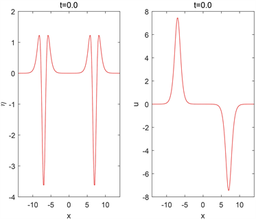
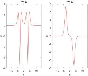
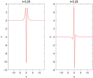
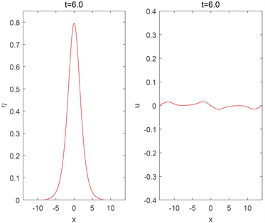
3.4. 有限时间爆破
这一个算例里面,取四个参数 , , , ,此时abcd Boussinesq系统退化为耦合的BBM方程组,并具有以下形式的行波解 [7]
(19)
取初始条件为
(20)
式中 ,计算区域取为 ,计算时间为 。 和u在爆破前不同时刻的数值解如图1所示。
 (a)
(a)
 (b)
(b)
 (c)
(c)
 (d)
(d)
Figure 1. The numerical solutions of and u at different times (before the blow-up)
图1. 和u在爆破前不同时刻的数值解
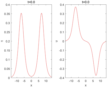
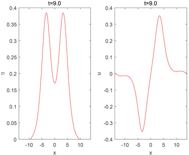
3.5. 孤立波的迎面碰撞
最后一个算例,考虑孤立波的迎面碰撞,取四个参数 , , , ,初始条件为
(21)
其中
(22)
。计算区域取为 , 和u在迎面碰撞前、后不同时刻的数值解如图2所示。
 (a)
(a)
 (b)
(b)
 (c)
(c)
 (d)
(d)
 (e)
(e)
Figure 2. The numerical solutions of and u at different times (head-on collision)
图2. 和u在迎面碰撞前后不同时刻的数值解
4. 结论
本文设计了一个数值求解abcd Boussinesq系统的高效数值方法,该方法首先通过引入人工变量来改写最初的模型,然后再将中心间断Galerkin-有限元方法应用到改写后的方程组,最后通过一系列的数值算例验证了该方法的高阶精度和可靠性。那么基于本文的工作,可以考虑将此类方法应用于更加复杂的非线性、色散浅水波模型的数值模拟。
基金项目
重庆市教育委员会科学技术研究项目(KJQN202200725)。
文章引用
夏有伟,程用平. abcd Boussinesq系统的高阶中心间断Galerkin-有限元方法
High Order Central Discontinuous Galerkin-Finite Element Methods for the abcd Boussinesq System[J]. 应用数学进展, 2023, 12(10): 4288-4299. https://doi.org/10.12677/AAM.2023.1210422
参考文献
- 1. Boussinesq, J. (1871) Théorie de l’intumescence liquide appelée onde solitaire ou de translation se propageant dans un canal rectangulaire. Comptes Rendus de l’Acadmie de Sciences, 72, 755-759.
- 2. Cheng, K., Feng, W., Gottlieb, W. and Wang, C. (2014) A Fourier Pseudospectral Method for the “Good’’ Boussinesq Equation with Second-Order Temporal Accuracy. Numerical Methods for Partial Differential Equations, 31, 202-224. https://doi.org/10.1002/num.21899
- 3. Li, X., Sun, W., Xing, Y. and Chou, C.-S. (2020) Energy Conserving Lo-cal Discontinuous Galerkin Methods for the Improved Boussinesq Equation. Journal of Computational Physics, 401, Article ID: 109002. https://doi.org/10.1016/j.jcp.2019.109002
- 4. Bona, J.L., Chen, M. and Saut, J.-C. (2002) Boussinesq Equations and Other Systems for Small-Amplitude Long Waves in Nonlinear Dispersive Media. I: Derivation and Linear Theory. Journal of Nonlinear Science, 12, 283-318. https://doi.org/10.1007/s00332-002-0466-4
- 5. Peregrine, D.H. (1966) Calculations of the Development of an Undular Bore. Journal of Fluid Mechanics, 25, 321-330. https://doi.org/10.1017/S0022112066001678
- 6. Bona, J.L., Dougalis, V.A. and Mitsotakis, D.E. (2007) Numer-ical Solutions of KdV-KdV Systems of Boussinesqequations: I. The Numerical Scheme and Generalized Solitary Waves. Mathmatics and Computers in Simulation, 74, 214-228. https://doi.org/10.1016/j.matcom.2006.10.004
- 7. Burtea, C. and Courtès, C. (2019) Discrete Energy Estimates for the abcd-Systems. Communications in Mathematical Sciences, 17, 243-298. https://doi.org/10.4310/CMS.2019.v17.n1.a10
- 8. Sun, J., Xie, S. and Xing, Y. (2022) Local Discontinuous Ga-lerkin Methods for the abcd Nonlinear Boussinesq System. Communications on Applied Mathematics and Computation, 4, 381-416. https://doi.org/10.1007/s42967-021-00119-4
- 9. Liu, Y., Shu, C.-W., Tadmor, E. and Zhang, M. (2007) Central Discontinuous Galerkin Methods on Overlapping Cells with a Nonoscillatory Hierarchical Reconstruction. SIAM Journal on Numerical Analysis, 45, 2442-2467. https://doi.org/10.1137/060666974
- 10. Liu, Y., Shu, C.-W., Tadmor, E. and Zhang, M. (2008) L2 Stability Anal-ysis of the Central Discontinuous Glerkin Method and a Comparison between the Central and Regular Discontinuous Galerkin Methods. ESAIM: Mathematical Modelling and Numerical Analysis, 42, 593-607. https://doi.org/10.1051/m2an:2008018
- 11. Liu, Y., Shu, C.-W., Tadmor, E. and Zhang, M. (2011) Central Local Discontinuous Galerkin Methods on Overlapping Cells for Diffusion Equations. ESAIM: Mathematical Modelling and Numerical Analysis, 45, 1009-1032. https://doi.org/10.1051/m2an/2011007
- 12. Liu, Y. (2005) Central Schemes on Overlapping Cells. Journal of Computational Physics, 209, 82-104. https://doi.org/10.1016/j.jcp.2005.03.014
- 13. Cockburn, B. and Shu, C.-W. (1989) TVB Runge-Kutta Local Pro-jection Discontinuous Galerkin Finiteelement Method for Conservation Laws II: General Framework. Mathematics of Computation, 52, 411-435. https://doi.org/10.1090/S0025-5718-1989-0983311-4
- 14. Cockburn, B., Hou, S. and Shu, C.-W. (1990) The Runge-Kutta Local Projection Discontinuous Galerkin Finiteelement Method for Conservation Laws IV: The Multidi-mensional Case. Mathematics of Computation, 54, 545-581. https://doi.org/10.1090/S0025-5718-1990-1010597-0
- 15. Shu, C.-W. (2016) Discontinuous Galerkin Methods for Time-Dependent Convection Dominated Problems: Basics, Recent Developments and Comparison with Other Methods. In: Barrenechea, G., Brezzi, F., et al., Eds., Building Bridges: Connections and Challenges in Modern Approaches to Numerical Partial Differential Equations, Springer, Berlin, 369-397. https://doi.org/10.1007/978-3-319-41640-3_12
- 16. Gottlieb, S., Shu, C.-W. and Tadmor, E. (2001) Strong Stabil-ity-Preserving High-Order Time Discretization Methods. SIAM Review, 43, 89-112. https://doi.org/10.1137/S003614450036757X
- 17. Chen, M. (1998) Exact Traveling-Wave Solutions to Bidirec-tional Wave Equations. International Journal of Theoretical Physics, 37, 1547-1567. https://doi.org/10.1023/A:1026667903256
NOTES
*通讯作者。