一类混合型积分微分方程的数值解法 A Numerical Solution of Mixed Integral Differential Equations

doi:10.12677/AAM.2018.77090

Advances in Applied Mathematics
Vol.07 No.07(2018), Article ID:25820,9 pages
10.12677/AAM.2018.77090

A Numerical Solution of Mixed Integral Differential Equations

Yang Liu, Yulan Wang

●How to Cite this Article

Inner Mongolia University of Technology, Hohhot Inner Mongolia

Received: Jun. 16^th, 2018; accepted: Jul. 4^th, 2018; published: Jul. 11^th, 2018

ABSTRACT

Polynomial approximation in the mathematical analysis and numerical approximation theory has an important position; it has been widely used in engineering calculation and the actual life. And the study of the numerical method for solving the integral differential equation is one of the important subjects exists in every field. This paper mainly based on Legendre polynomial rebuilding the reproducing kernel, through the “Gram-Schmidt”, the approximate solution of the equation is given. At the same time, it gives three numerical examples of Volterra-Fredholm integral differential equation. Compared with the traditional methods of reproducing kernel, we further verified that our method was effective and had high precision. All numerical calculations are given by the Mathematica 8.0 software.

Keywords:Legendre Polynomials, Reproducing Kernel, Numerical Solution, Volterra-Fredholm Integral Differential Equation

一类混合型积分微分方程的数值解法

刘杨，王玉兰

内蒙古工业大学，内蒙古呼和浩特

收稿日期：2018年6月16日；录用日期：2018年7月4日；发布日期：2018年7月11日

摘要

多项式逼近在数学分析和数值逼近理论中具有重要的地位，它已广泛应用于工程计算和实际生活中。而且关于积分微分方程数值解法的研究一直是存在于各领域的重要课题。本文主要基于Legendre多项式重新构建再生核，通过Gram-Schmidt给出方程的近似解。同时，给出三个Volterra-Fredholm积分微分方程的数值算例，与传统的再生核方法进行数值比较，进一步验证了我们方法是有效的，且具有很高的精度。所有数值计算都是通过数学软件Mathematica8.0给出。

关键词 :Legendre多项式，再生核，数值解，Volterra-Fredholm型积分微分方程

This work is licensed under the Creative Commons Attribution International License (CC BY).

http://creativecommons.org/licenses/by/4.0/

1. 引言

当今社会发展迅速，逼近的思想几乎渗透到所有生产生活领域。在当今这个时代，函数逼近理论更是不可或缺，它不仅可以研究各个函数的性质、而且在函数零点的研究、数值积分的构造及求解微分方程、积分方程等方面都有广泛的应用。

多项式逼近理论是数学分析中非常有研究价值的一个课题。一般地，而函数思想就是用较简单的函数近似代替定区间上较为复杂的连续函数，但由于计算机在运算方面存在局限性，我们通常选取多项式、有理分式或三角多项式逼近去计算复杂函数值。这是因为它们的实际意义相对较大，特别是多项式。多项式不仅计算上比较容易，求导、求积分相对简单。因此，用多项式逼近函数在数值近似理论、工程计算以及生产生活中都有着广泛的应用。

长期以来，积分微分方程深受各国学者的关注 [1] - [11] 。因为此类方程常常成功地运用在高能物理及生物医学工程等方面，帮助描述相关物理现象及规律。那么如何求解这类方程就变成了必不可少的研究课题。但对于积分微分方程其精确解往往通过较复杂的函数构造的，即使这类方程可以求其精确解，但也是少数，而且无法用数值表示，特别是某些非线性的方程。所以研究此类方程的数值解尤为必要。

本文基于Legendre多项式，重新构造再生核，并通过再生核相关理论进一步给出混合积分微分方程的数值解。为此我们考虑下列混合型积分微分方程：

${\begin{cases} q_{1} (x) u^{(n)} (x) + q_{2} (x) u^{(n - 1)} (x) + q_{3} (x) u (x) + \int_{0}^{x} k_{1} (t, x) u (t) d t + \int_{0}^{1} k_{2} (t, x) u (t) d t = f (x), 0 \leq x \leq 1 \\ u^{(i)} (0) = α_{i}, u^{(j)} (1) = β_{j}, 0 \leq i, j \leq n - 1. \end{cases}$ (1)

其中 $q_{1} (x), q_{2} (x), q_{3} (x), k_{1} (t, x), k_{2} (t, x), f_{1} (x)$ 为已知的连续函数， $α_{i}, β_{j}$ 为常数， $u (x)$ 为未知函数。

2. 勒让德多项式

当区间为 $[- 1, 1]$ ，权函数 $ρ (x) = 1$ 时，对 ${1, x, \dots, x^{n}, \dots}$ 正交化处理得到的多项式称为Legendre多项式．记 ${P_{n} (x)}_{n = 0}^{\infty}$ ，这些多项式满足

$\int_{- 1}^{1} P_{n} (x) P_{m} (x) d x = \frac{2}{2 n + 1},$ (2)

为了使这些多项式投射到 $[0, 1]$ 区间上，我们通过作变换： $x = 2 t - 1$ ，则 $P_{n} (x) = P_{n} (2 t - 1)$ 称其为移位Legendre多项式。记 $P_{n} (2 t - 1) = L_{n} (t)$ ，显然 ${L_{n} (t)}_{n = 0}^{\infty}$ 在区间 $[0, 1]$ 上带权函数 $ρ (x) = 1$ 正交，即

$\int_{0}^{1} \sqrt{2 n + 1} L_{n} (t) \sqrt{2 n + 1} L_{m} (t) d t = 1 .$ (3)

$L_{i} (t)$ 有如下的递推关系

$\begin{array}{l} L_{i + 1} (t) = \frac{(2 i + 1) (2 - 1)}{i + 1} L_{i} (t) - \frac{i}{i + 1} L_{i - 1} (t), i = 1, 2, \dots \\ L_{0} (t) = 1, L_{1} (t) = 2 t - 1. \end{array}$ (4)

n阶移位的Legendre多项式的一般表达式为：

$\begin{array}{l} L_{n} (t) = \sum_{i = 0}^{n} {(- 1)}^{n + i} \frac{(n + i)! t^{i}}{(n - i)! (i)!^{2}}, \\ L_{n} (0) = {(- 1)}^{(n)}, L_{n} (1) = 1 . \end{array}$ (5)

经过线性变换后，我们令 $Q_{n} (x) = \sqrt{2 n + 1} L_{n} (t)$ ， ${Q_{n} (x)}_{i = 1}^{n}$ 是标准正交基。

3. 造核

定义：设H是Hilbert空间，B是某个数集，若存在二元函数 $K (s, t)$ ，使得 $\forall s \in B$ ，都有 $f (s) = 〈 f (t), K_{s} (t) 〉, \forall f (t) \in H, K_{s} (t) \in H$ ，则称 $K (s, t)$ 为H的再生核核，此时H为再生核空间。

引理：H是有限维的Hilbert空间， ${e_{i} (t)}_{i = 1}^{n}$ 是H的标准正交基，即

$〈 e_{i} (t), e_{j} (t) 〉 = δ_{i j} = {\begin{cases} 0 (i \neq j) \\ 1 (i = j) \end{cases},$ (6)

则有 $K (s, t) = \sum_{i = 1}^{n} e_{i} (t) e_{j} (s)$ 为H的再生核。

证明： $\forall f (t) = \sum_{i = 1}^{n} c_{i} e_{i} (t)$ ，故

$\begin{matrix} 〈 f (t), K_{s} (t) 〉 = 〈 \sum_{i = 1}^{n} c_{i} e_{i} (t), \sum_{j = 1}^{n} e_{i} (t), e_{i} (s) 〉 \\ = \sum_{i = 1}^{n} c_{i} 〈 e_{i} (t), \sum_{j = 1}^{n} e_{j} (t) e_{j} (s) 〉 \\ = \sum_{i = 1}^{n} c_{i} e_{i} (s) \\ = f (s) . \end{matrix}$ (7)

得证。

3.1. 构造再生核空间(RKM)

由上述定理知H是有限维的Hilbert空间， ${Q_{n} (x)}_{i = 1}^{n}$ 是H的标准正交基，则 $K (x, y) = \sum_{i = 1}^{n} Q_{n} (x) Q_{m} (y)$ 为H的再生核。具体表达式如下：

$K (x, y) = 1 + 3 (2 x - 1) (2 y - 1) + 5 \frac{3 {(2 x - 1)}^{2}}{2} \frac{3 {(2 y - 1)}^{2}}{2} + \dots + (2 n + 1) Q_{n} (x) Q_{m} (y) .$ (8)

3.2. 近似解的表示

对于方程(1)中非齐次边值条件需齐次化处理。

令 $v (x) = u (x) + a_{1} + a_{2} x + a_{3} x^{2} + \dots + a_{n} x^{n - 1}$ ，则方程(1)转化为：

${\begin{cases} q_{1} (x) v^{(n)} (x) + q_{2} (x) v^{(n - 1)} (x) + q_{3} (x) v (x) + \int_{0}^{x} k_{1} (t, x) v (t) d t + \int_{0}^{1} k_{2} (t, x) v (t) d t = f (x), 0 \leq x \leq 1 \\ v^{(i)} (0) = 0, v^{(j)} (1) = 0, 0 \leq i, j \leq n - 1 . \end{cases}$ (9)

对于齐次化后的初边值条件，我们放到再生核空间中，放核过程见文献 [12] 。

完全系的构造

令 $A v = q_{1} (x) v^{(n)} (x) + q_{2} (x) v^{(n - 1)} (x) + q_{3} (x) v (x) + \int_{0}^{x} k_{1} (t, x) v (t) d t + \int_{0}^{1} k_{2} (t, x) v (t) d t,$ (10)

方程(9)转化为

$(A v) (x) = f (x) .$ (11)

其中A是线性可逆算子。

令 $ψ_{i} (x) = {A_{y} K (x, y) |}_{y = x_{i}}, i = 0, 1, 2, \dots$ 且 $〈 ψ_{j} (x), ψ_{i} (x) 〉 = {A_{x} A_{y} K (x, y) |}_{x = x_{j}}, i, j = 1, 2, \dots$ 此时， ${ψ_{i} (x)}_{i = 1}^{\infty}$ 是完全函数系。具体证明见文献 [12] 。对此完全系做Gram-Schimdt，我们可以得到标准正交基 ${{\tilde{ψ}}_{i} (x)}_{i = 1}^{\infty}$ ， ${\tilde{ψ}}_{i} (x) = \sum_{k = 1}^{i} β_{i k} ψ_{i} (x), i = 1, 2, \dots$ 其中 $β_{i k}$ 为正交化系数。

定理：设 $v (x)$ 为方程(11)的解，则 $v (x) = \sum_{i = 1}^{\infty} \sum_{k = 1}^{i} {\tilde{β}}_{i k} f (x_{k}) {\tilde{ψ}}_{i} (x)$ 。

证明：

$\begin{matrix} v (x) = \sum_{i = 1}^{\infty} 〈 v, {\tilde{ψ}}_{i} 〉 {\tilde{ψ}}_{i} (x) \\ = \sum_{i = 1}^{\infty} 〈 v, \sum_{k = 1}^{i} β_{i k} ψ_{k} 〉 {\tilde{ψ}}_{i} (x) \\ = \sum_{i = 1}^{\infty} \sum_{k = 1}^{i} {\tilde{β}}_{i k} 〈 v, A_{y} K (x, y) 〉 {\tilde{ψ}}_{i} (x) \\ = \sum_{i = 1}^{\infty} \sum_{k = 1}^{i} {\tilde{β}}_{i k} A v (x_{k}) {\tilde{ψ}}_{i} (x) \\ = \sum_{i = 1}^{\infty} \sum_{k = 1}^{i} {\tilde{β}}_{i k} f (x_{k}) {\tilde{ψ}}_{i} (x) . \end{matrix}$ (12)

方程的近似解为：

$v_{n} (x) = \sum_{i = 1}^{n} \sum_{k = 1}^{i} {\tilde{β}}_{i k} f (x_{k}) {\tilde{ψ}}_{i} (x) .$ (13)

故方程(1)的近似解为

$u_{n} (x) = \sum_{i = 1}^{n} \sum_{k = 1}^{i} {\tilde{β}}_{i k} f (x_{k}) {\tilde{ψ}}_{i} (x) - a_{1} - a_{2} x - a_{3} x^{2} - \dots - a_{n} x^{n - 1} .$ (14)

4. 数值算例

算例1 (见文献 [13] )

${\begin{cases} x u^{″} (x) - x u^{'} (x) + 2 u (x) - \int_{0}^{x} (x - t) u (t) d t - \int_{0}^{1} (x + t) u (t) d t = \frac{1}{12} x^{4} - \frac{1}{6} x^{3} - \frac{1}{2} x^{2} - \frac{13}{6} x + \frac{17}{12}, \\ 0 < x < 1, 0 < t < 1, \\ u (0) = 1, u (1) = 1 . \end{cases}$

精确解 $u (x) = 1 + x - x^{2}$ 。

本算例我们将基于Legendre多项式重新构建再生核函数与传统的再生核法进行数值计算得到的数值结果见图1，图2及表1，从图表中我们可以看出改进的再生核方法绝对误差更小，精度更高。

算例2 (见文献 [13] )

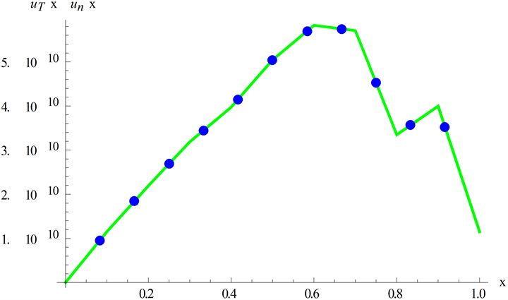
Figure 1. Absolute error of the improved RKM of Example 1

图1. 改进再生核方法的绝对误差(例1)

Figure 2. Absolute error of the traditional RKM of Example 1

图2. 传统再生核方法的绝对误差(例1)

${\begin{cases} x^{2} u^{(4)} (x) - u^{″} (x) + u^{'} (x) - \int_{0}^{x} (x - t) u (t) d t + 2 \int_{0}^{1} (x + t) u (t) d t = - \frac{1}{12} x^{4} - \frac{1}{2} x^{2} + \frac{14}{3} x - \frac{1}{2}, \\ 0 < x < 1, 0 < t < 1, \\ u (0) = 1, u^{'} (0) = 0, u (1) = 2, u^{'} (1) = 2. \end{cases}$

精确解 $u (x) = 1 + x - x^{2}$ 。

此题我们仍然采用两种处理方式，因两种方法的绝对误差数量级相差不大，我们在此将两者的绝对误差放在同一图3中，黑色曲线代表改进的再生核方法，红色曲线代表传统的再生核方法，从图中我们可以看出两种方法都具有较小误差，但是改进后的再生核方法精确度更高。

Table 1. Absolute error of two regenerated kernel methods of Example 1

表1. 两种再生核方法的绝对误差的计算结果(例1)

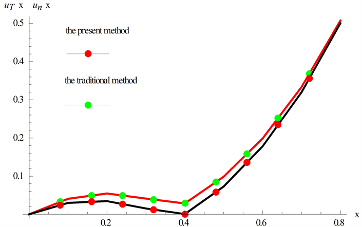
Figure 3. Absolute error of two RKM of Example 2

图3. 两种再生核方法的绝对误差的计算结果(例2)

算例3 (见文献 [14] )

${\begin{cases} u^{″} (x) + \frac{1}{\sqrt{x}} u^{'} (x) + \frac{1}{x} u (x) + \int_{0}^{x} (t + x) u (t) d t + \int_{0}^{1} t x u (t) d t - \frac{1}{1 + \sin (u^{2} (x))} - e^{u^{9} (x)} + u^{11} (x) = f (x), \\ 0 < x < 1, \\ u (0) = 0, u (1) = 0. \end{cases}$

精确解 $u (x) = (x - x^{2}) \sin (x)$ 。

图4，图5代表改进的再生核方法和传统的再生核方法的绝对误差，从图中我们可以看出改进的再生核方法精度更高，具体的数值结果见表2。

Figure 4. Absolute error of the improved RKM of Example 3

图4. 改进再生核方法的绝对误差(例3)

Figure 5. Absolute error of the traditional RKM of Example 3

图5. 传统再生核方法的绝对误差(例3)

Table 2. Absolute error of two regenerated kernel methods of Example 3

表2. 两种再生核方法的绝对误差的计算结果(例3)

5. 结论

本文基于Legendre多项式重新构建再生核空间，并通过Gram-Schmidt正交化进一步给出方程的近似解。同时我们也通过求解3个混合型的Volterra-Fredholm积分微分方程的数值算例，与传统的再生核方法进行数值比较，进一步验证了我们的方法是有效且可行的。本文的所有数值计算都是通过数学软件Mathematica8.0给出。

致谢

感谢王玉兰老师的支持与帮助。

文章引用

刘杨,王玉兰. 一类混合型积分微分方程的数值解法
A Numerical Solution of Mixed Integral Differential Equations[J]. 应用数学进展, 2018, 07(07): 749-757. https://doi.org/10.12677/AAM.2018.77090

参考文献

1. Beyrami, H. and Lotfi, T. (2017) Stability and Error Analysis of the Reproducing Kernel Hilbert Space Method for the Solution of Weakly Singular Volterra Integral Equation on Graded Mesh. Applied Numerical Mathematics, 120, 197-214.
https://doi.org/10.1016/j.apnum.2017.05.010

2. Guo, B.B., Jiang, W. and Zhang, C.P. (2017) A New Numerical Method for Solving Nonlinear Fractional Fokker-Planck Differential Equations. Journal of Computational and Nonlinear Dynamics, 12, 051004.
https://doi.org/10.1115/1.4035896

3. Abu Arqub, O. (2017) Fitted Reproducing Kernel Hilbert Space Method for the Solu-tions of Some Certain Classes of Time-Fractional Partial Differential Equations Subject to Initial and Neumann Boundary Conditions. Computers Mathematics with Applications, 73, 1243-1261.
https://doi.org/10.1016/j.camwa.2016.11.032

4. Du, M.J., Wang, Y.L. and Chaolu, T. (2017) Reproducing Kernel Method for Numerical Simulation of Down Hole Temperature Distribution. Applied Mathematics and Computation, 97, 19-30.
https://doi.org/10.1016/j.amc.2016.10.036

5. Henderson, J. and Kunkel, C.J. (2008) Uniqueness of Solution of Linear Non-local Boundary Value Problems. Applied Mathematics Letter, 21, 1053-1056.
https://doi.org/10.1016/j.aml.2006.06.024

6. Cui, M.G. (2010) An Efficient Computational Method for Linear Fifth-Order Two-Point Boundary Value Problems. Journal of Computational and Applied Mathematics, 234, 1551-1558.
https://doi.org/10.1016/j.cam.2010.02.036

7. Wang, Y.L., Chaolu, T. and Chen, Z. (2010) Using Reproducing Kernel for Solving a Class of Singular Weakly Nonlinear Boundary Value Problems. International Journal of Computer Mathematics, 87, 367-380.
https://doi.org/10.1080/00207160802047640

8. Wang, W.Y. and Han, B. (2013) Inverse Heat Problem of Determining Time-Dependent Source Parameter in Reproducing Kernel Space. Nonlinear Analysis Real World Applications, 14, 875-887.
https://doi.org/10.1016/j.nonrwa.2012.08.009

9. Ketabchi, R., Mokhtari, R. and Babolian, E. (2015) Some Error Estimates for Solving Volterra Integral Equations by Using the Reproducing Kernel Method. Journal of Computational and Applied Mathematics, 273, 245-250.
https://doi.org/10.1016/j.cam.2014.06.016

10. Jiang, W. and Chen, Z. (2013) Solving a System of Linear Volterra Integral Equations Using the New Reproducing Kernel Method. Applied Mathematics and Computation, 219, 10225-10230.
https://doi.org/10.1016/j.amc.2013.03.123

11. Abu Arqub, O. (2016) The Reproducing Kernel Algorithm for Handling Dif-ferential Algebraic Systems of Ordinary Differential Equations. Mathematical Methods in the Applied Sciences, 39, 4549-4562.
https://doi.org/10.1002/mma.3884

12. Jiang, W. and Tian, T. (2015) Numerical Solution of Nonlinear Volter-raintegro-Differential Equations of Fractional Order by the Reproducing Kernel Method. Applied Mathematical Modelling, 39, 4871-4876.
https://doi.org/10.1016/j.apm.2015.03.053

13. Wang, W.M. (2006) An Algorithm for Solving the High-Order Nonlinear Volterra-Fredholm Integro-Differential Equation With Mechanization. Applied Mathematics and Computation, 172, 1-23.
https://doi.org/10.1016/j.amc.2005.01.116

14. Wang, Y.L., Chaolu, T. and Pang, J. (2009) New Algorithm for Second-order Boundary Value Problems of Integro-Differential Equations. Journal of Computational and Applied Mathematics, 229, 1-6.
https://doi.org/10.1016/j.cam.2008.10.040

期刊菜单