Advances in Applied Mathematics
Vol.
12
No.
08
(
2023
), Article ID:
71153
,
16
pages
10.12677/AAM.2023.128367
浅水波方程的高阶保正Well-Balanced ADER间断Galerkin格式
周翔宇,张志壮,钱守国,李刚*
青岛大学数学与统计学院,山东 青岛
收稿日期:2023年7月26日;录用日期:2023年8月18日;发布日期:2023年8月24日

摘要
本文针对具有不规则几何形状和非平坦底地形的浅水波方程,引入了保正高阶ADER间断Galerkin方法,该方法能准确地保持静水的稳态。为了满足well-balanced的性质,我们提出了well-balanced的数值通量,并基于分解算法将数值解分解为两部分,构造了一种新的源项近似,并相应地将源项近似分解为两部分。此外,还引入了一个简单的保正限制器,从而在干湿锋面附近提供高效和鲁棒性的模拟。大量的数值实验也表明,所得到的格式s能够准确地捕捉静止稳定状态下湖泊的小扰动,保持水面高度的非负性,同时保持光滑解的真正高阶精度。
关键词
浅水波方程,ADER方法,间断Galerkin格式,保证格式,微分变换过程,全离散

High Order Well-Balanced ADER Discontinuous Galerkin Scheme for Shallow Water Wave Equations
Xiangyu Zhou, Zhizhuang Zhang, Shouguo Qian, Gang Li*
School of Mathematics and Statistics, Qingdao University, Qingdao Shandong
Received: Jul. 26th, 2023; accepted: Aug. 18th, 2023; published: Aug. 24th, 2023

ABSTRACT
In this paper, we introduce positivity-preserving high order ADER discontinuous Galerkin Methods for the shallow water equations with irregular geometry and a non-flat bottom topography, which maintain the still water steady state exactly. To achieve the well-balanced property, we propose the well-balanced numerical fluxes, and construct a novel source term approximation by decomposing the numerical solutions into two parts based on decomposition algorithm, and resolving the approximation to the source term into two parts accordingly. Moreover, a simple positivity-preserving limiter is introduced in one dimension and then extended to two dimensions to provide efficient and robust simulations near the wetting and drying fronts. Extensive one and two dimensional simulations also indicate that the resulting schemes enjoy the ability to accurately capture small perturbations to the lake at rest steady state, maintain the non-negativity of the water height, and keep the genuine high order accuracy for smooth solutions at the same time.
Keywords:Shallow Water Wave Equations, ADER Approach, Discontinuous Galerkin Scheme, Positivity-Preserving Method, Differential Transformation Procedure, Fully-Discrete

Copyright © 2023 by author(s) and Hans Publishers Inc.
This work is licensed under the Creative Commons Attribution International License (CC BY 4.0).
http://creativecommons.org/licenses/by/4.0/


1. 引言
在本文中,我们主要的工作是构造非平坦底部地形上的浅水波方程(SWEs)的保正well-balanced性质的间断Galerkin格式,该方程具体形式如下 [1] [2] [3] [4] :
(1)
在上式中,h为水深,u为水深平均速度,b为水底地形。g是重力加速度常数。
浅水波方程(1)属于双曲守恒律的一种,并且其静水稳态解由下式给出:
(2)
其中源项与通量梯度完全平衡。这种平衡律的数值模拟,包括非平坦底部地形上的非线性浅水波方程,有一个主要的问题:标准数值方法可能无法在离散水平上保持稳态下通量梯度和源项之间的平衡,并且可能在稳态附近产生伪振荡。Well-balanced方法旨在克服这一问题,并且在稳态(或接近稳态)解决格式下表现良好。对于非线性SWEs,已经有多种方法被提出并应用,其中包括 [5] - [12] 及其参考文献。在相关问题的数值模拟中,另一个经常遇到的问题是对少水或无水地区的润湿和干燥情况的处理。典型的问题包括溃坝问题、洪波和爬高现象。数值上,在计算过程中可能会产生负值,这可能会带来额外的困难。有许多现有的保正方法可以克服这一困难,关于这些方法我们参考了文献 [13] - [18] 。
上述对浅水波方程的所有工作都是在有限差分法或有限体积法的基础上进行的。在过去的几十年中,高阶有限元Galerkin(DG)方法在求解包含双曲型守恒律的偏微分方程方面得到了广泛的关注。
近十多年来,高阶时间和空间任意导数方法在求解对流占优问题中得到了广泛的关注。Toro和合作者最初在双曲守恒律的有限体积格式背景下提出了ADER格式 [19] [20] [21] 。格式 [19] [20] [21] 是单步、单级和全离散的。后来,Dumbser和Munz [22] [23] [24] 提出了一种采用单阶段ADER方法 [19] [20] [21] 的DG方法,用于时间离散化。随后,Dumbser等人对该方法进行了一系列研究 [25] [26] [27] [28] 。
DG方法 [25] [26] [27] [28] 的关键是构造高阶数值通量。网格间状态以时间泰勒级数展开的形式表示,其中时间导数由使用控制PDE的空间导数表示。该程序被称为Cauchy-Kowalewski程序(在文献中也称为Lax-Wendroff程序 [29] )。此外,还需要求解网格间的广义黎曼问题,以获得状态本身及其空间导数。然而,Cauchy-Kowalewski方法非常繁琐,尤其是在求解高维问题的时候。因此,CauchyKowalewski程序的替代或简化是非常有意义的。值得注意的是,Dumbser和Munz [30] 提出了一种高效的Cauchy-Kowalewski过程算法。最近,Dumbser等人 [31] ,Duan和Tang [32] 采用局部连续时空Galerkin预测方法 [33] 来取代DG方法框架下的Cauchy-Kovalewski过程。
Galerkin (DG)方法是一类以高阶间断分段多项式空间作为测试函数空间的有限元方法 [34] [35] [36] 。半离散DG方法(也称为RKDG方法)使用间断的分段多项式空间作为数值解和测试函数空间,并通过TVD Runge-Kutta格式进行稳定的高阶时间积分 [37] - [42] 。Qian [43] 设计了几何形状不规则的明渠浅水波方程的高阶保正平衡方法。
最近,ADER方法由Toro和Titarev引入到有限体积格式中,该方法通过完全离散的一步公式获得空间和时间上任意高阶精度。原始版本的ADER方法在空间和时间上使用截断的Taylor展开,并通过Cauchy-Kovalevskaya (C-K)过程 [44] 将时间导数替换为空间导数,但是该过程不能处理刚性源项。为了克服这些问题,ADER-DG方法用局部时空DG预测器取代C-K过程 [45] 。因此,单步公式只需要逐点计算通量和源项,这样就极大地减少了空间元素之间的模板依赖,并允许几乎完美的并行化。
在本文中,我们构造了湖处于静止稳态的SWEs的高阶良好平衡的ADER-DG方法,并用微分变换代替C-K过程。为了达到良好的平衡性能,我们建议结合基于流体静力重建思想的数值通量,以及一种新的源项近似和分解算法。所得到的DG方法在保持湖泊静止稳态的well-balanced特性的同时,又保持了光滑解的高阶精度。
本文结构如下:在第2节中,我们提出了保正平衡的ADER-DG方法。第3节给出了一些数值算例来验证所提出的ADER-DG方法的性能。最后,第4节给出结论。
2. ADER-DG方法
在本节中,我们构造了浅水波方程的高阶良好平衡的ADER-DG方法(1)。为了准确地保持静水稳态(2),我们基于流体静力重建技术构建了well-balanced的数值通量,并提出了一种新的基于分解算法的源项近似。
2.1. 符号记法
首先将空间区间 离散成N个单元 。每个单元格的中心是 ,单元格 的大小记为 ,最大网格大小记为 。符号 表示时空控制体积, 为时间间隔。在这里,我们取近似解空间如下:
(3)
其中 表示 上k次以下的时空多项式集合。注意, 中的函数允许在元件界面上具有间断。此外,我们使用 表示函数 在元素界面 处的算术平均值。
2.2. 微分变换过程
在本节中,我们将介绍一种基于将微分方程转化为其时空序列展开解的系数递推关系的方法,称为微分变换法(DTM) [46] 。值得注意的是,该方法在评估C-K过程时更加简洁高效 [47] 。为方便起见,我们首先考虑一维平流方程
(4)
将 的初始条件展开为泰勒多项式
(5)
接下来,我们假设解可以表示为每个时空域内的以下多项式
(6)
微分变换 的形式是这样的
(7)
将(6)代入平流式(4),可得递归关系如下:
(8)
因此,从式(5)中的初始微分变换 开始,反复重复式(8),得到任意时刻的微分变换。因此,我们可以通过泰勒级数展开(6)得到平流方程(4)的解,即任意高阶解。
随后,我们考虑了浅水波方程的微分变换方法(13)。我们将 的初始条件投影到分段多项式空间 中,得到 ,其形式为
(9)
与Runge-Kutta DG方法不同,我们通过k次的时空多项式在每个时空域 内寻找浅水波方程(13)的数值解,如下所示
(10)
与2.2节类似,我们将(10)代入(45),得到浅水波方程(12)的递推关系如下:
(11)
其中
因此,将初始微分变换 和 代入(11),得到微分变换 ,并利用(10)得到在时空域 上的近似。
2.3. ADER-DG方法的构建
在本节中,我们将利用2.2节中的微分变换过程构建SWEs(1)的ADER-DG方法。
首先,我们将原控制方程(1)改写为
(12)
我们将源项 按照 [48] [49] 中的方法改写为动量方程中的等效形式 。
为了便于表示,我们引入了可以将(12)改写为紧致向量形式的符号
(13)
其中 和 分别表示保守变量、物理通量和几何源项。
式(13)与任意空间测试函数 的乘法并使用 上的部分积分产生以下弱形式
这里,为了便于表示,我们将物理通量写作一个二元函数 。
求解(13)的全离散ADER-DG方法定义如下:对于所有测试函数 且 ,从 出发,解 满足
(14)
这里用数值通量 来近似网格之间物理通量的时间积分,即 。其中 数值通量与简单的Lax-Friedrichs通量一致
(15)
其中
. (16)
其中 为雅可比矩阵 的特征值,其具体形式为
. (17)
2.4. 平衡良好的数值通量
请注意,在前一小节中提出的ADER-DG方法(45)不具有良好的平衡特性。在本节中,我们提出了对数值通量的修正,目的是准确地保持稳态(2)。
为了保持正性(如第2.14节所述),我们还在时间步长 上引入了新的网格边界值:
(18)
其中
在(2)中满足稳定性。
现在,让我们讨论平衡的数值通量。在(15)定义的Lax-Friedrichs数值通量 中,附加项 对数值黏度起到了作用,这是非线性守恒律所必需的。然而,它们可能破坏稳态的良好平衡特性。因此,我们将该通量(15)修改为
(19)
这里我们将通量项的第一个分量从 修改为 以便在第2.14节中解释保正性。
2.5. 源项近似
接下来,我们给出源项积分的高阶平衡近似,其形式为
(20)
其中 表示源项的第二分量。我们可以进一步把这个积分分解为
(21)
其中项 分别用它们的数值近似值 代替。此外,将 的边界值替换为它们在网格面处的平均值,记为 ,与稳态时的数值通量(51)一致。
2.6. 斜率限制器
对于双曲守恒律系统,当解包含间断点时,ADER-DG方法通常与斜率限制程序相结合,以压缩间断点附近可能出现的振荡。文献中有许多不同的斜率限制器选择,本文我们考虑经典的全变分有界(TVB)限制器 [50] 。
标准限制器可能与良好平衡性质相冲突,我们根据 [51] 中提出的思想提出了一个良好平衡限制器程序。未知 上的标准TVB限制器包括两个步骤。第一步是根据网格平均值 和网格边界值 来检查单元 中是否需要任何限制。第二步是对该单元 中的变量 应用TVB限制器。在提出的平衡斜率限制程序中,我们将首先根据单元平均值 和 来检查是否需要限制。如果单元 被标记为需要限制,则实际的TVB限制器像往常一样应用于 。注意 在静水稳态(2)时变为常数,因此在达到稳态时不施加限位器,保持了良好的平衡性质。
2.7. 均衡格式概要
我们提出的浅水波方程(1)的良好平衡ADER-DG方法由式(45)给出,其中的数值通量定义在式(51)中,源项近似在上文中已经给出。综合前面各小节的结果,可以很直观地证明如下结果:
命题1 上述浅水波方程(1)的ADER-DG方法可以保持稳态解(2)的well-balanced性。
证明 在稳态(2)时,我们有
我们只需要证明包含源项的动量方程的平衡性。将方程中的通量项用 表示。对于式(51)中给出的数值通量,式(45)左侧的数值近似为
(22)
由于 ,源项近似变成
注意这个等式
并由此我们得出结论,通量和源项近似在静水稳态时相互平衡,从而得到期望的良好平衡特性。
2.8. Positivity-Preserving方法
在 [52] 中,Zhang和Shu提出了设计双曲守恒律的高阶最大原理保持方法的框架。从那时起,该方法得到了许多关注,并被广泛应用,包括 [53] 中的浅水波方程。结果表明,在合适的CFL条件下,能保持水高的非负性而不影响质量守恒,并能保持通解的高阶精度。在这里,我们将探讨这种方法在第2节中为浅水波方程提出的平衡良好的ADER-DG方法中的应用。
如 [54] 所述,实现这一目标的关键组成部分是以下两项:该方法一阶版本的正性,以及与高阶方法耦合的简单保正限制器。在建立之后,我们只考虑简单的欧拉时间离散化,同样的结果可以推广到多步和TVD高阶龙格–库塔方法。考虑平衡良好的ADER-DG方法(45)与(51)中定义的数值通量,取测试函数 导致湿截面的单元平均更新如下
(23)
其中
(24)
并且有 。为方便起见,设 。为了不丧失一般性,我们在本节中忽略下标 。该方法的一阶形式为
(25)
其数值通量定义为
(26)
其中 。
关于这种一阶方法的保正性,我们有如下引理:
引理2 在CFL条件 下,考虑具有数值通量(57)的一阶格式(56)。如果 是非负的,那么 也是非负的。
证明 格式(56)可写成
因此, 是 , 和 的线性组合,并且所有系数都是非负的,因为 , 。因此, 。
接下来,我们讨论高阶格式。我们参考 [54] 了解细节,这里只介绍主要思想。我们在区间 上引入N点( ) Legendre gaas-lobatto正交规则,用 ,表示这些正交点,在区间 上对应的正交权值 满足。由于求积对于k次多项式是精确的,我们有
(27)
按照 [55] 的方法,我们得到的结果是:
命题3 对于浅水波方程(1)的格式(45),我们设 为单元格 中的DG多项式。如果 和 都是非负的,则在CFL条件下 也是非负的:
(28)
证明我们把(58)代入(54),重写(54)通过加减 :
(29)
以及
(30)
(31)
注意到
(32)
可以清楚地看到 是 和 的线性组合,并且所有系数都是非负的,因为 (这也证明了我们在 的合适CFL条件下分别定义α和为(49)和(50)的原因。因此,我们得到 ,同样有 。由于 ,这两个CFL条件相同,也就是(59)。因此, ,因为它是 和 的凸组合。
我们在DG多项式 上采用了以下保正极限器 [56] [57] ,
(33)
并有
(34)
很容易观察到 ,该极限保持变量 的局部守恒。
我们计算修正的多项式 ,并在均衡方法中使用 代替 (45)。根据 [56] [57] 中的证明,我们可以验证在CFL条件下,与该保正限制器耦合的平衡方法是高阶精度、保正和质量守恒的
(35)
为了提高效率,只有当对下一个时间步长的初步计算产生负湿截面时,我们才实现时间步长限制(66)。
3. 数值结果
为了证明well-balanced的ADER-DG格式的良好性能,我们给出了几个标准的浅水波方程的数值算例的结果。在所有的算例中,CFL数和引力常数g分别取0.16和9.812。
3.1. 平坦底部的黎曼问题
在本节中,我们考虑包含平坦底部的干面积(即 )的黎曼问题。这些例子在 [58] 中使用过,这
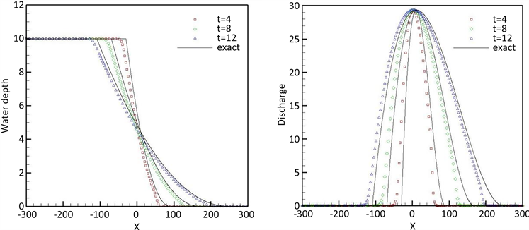
Figure 1. The numerical and exact solutions of the first Riemann problem at different time with 200 cells in Section 3.1: left: the water height h; right: the discharge hu
图1. 第3.1节中200个网格的第一黎曼问题在不同时间的数值解和精确解水高h (左)和水体动量hu (右)
里选择它们是为了证明我们的方法的保正能力。该例的计算域设置为[−300, 300],初始条件为
左侧为静水高度设为10,右侧为干区。该问题的解析解可在 [59] 中找到。我们用我们的平衡保正方法计算了这个问题,该方法具有简单的传输边界条件和200个均匀单元。 时刻的解如图1所示。我们还在这些图中绘制了精确的解,以便进行比较。我们可以观察到,数值结果很好地反映了精确解。
3.2. 抛物线碗
Sampson等人 [60] 推导出了具有抛物型底地形的一维浅水波方程的解析解。这为我们的数值方法提供了一个很好的测试用例。这个例子已在 [61] 中用于具有摩擦源项的浅水波方程。我们取抛物线底部:
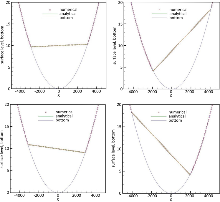
Figure 2. The water surface level in the parabolic bowl problem at different time in Section 3.2: top left: t = 1000; top right: t = 2000; bottom left: t = 3000; bottom right: t = 4000
图2. 第3.2节中抛物面碗问题不同时刻的水面水平:左上:t = 1000;右上:t = 2000;左下:t = 3000;右下:t = 4000
常数 和a下文定义。计算域设置为[−5000, 5000]。对于不含摩擦源项的浅水波方程,解析水面由式给出
其中 。干湿锋面的确切位置如图2所示:
3.3. 干燥河床的生成问题
我们首先考虑 [62] 中提出的平底 的数值实验。初始条件为
在这个例子中,干燥的河床会在两个方向相反的稀有波的中间产生。干层的生成使得这个例子很难用数值计算。将t = 1时刻得到的结果进行比较,正如图3可以观察到的那样,目前的格式在两个稀疏波之间留下了一个小的湿区。通过图中绘制出的精确解我们可以清晰的观察到,数值结果具有良好的保正性,并且很好地反映了精确解。
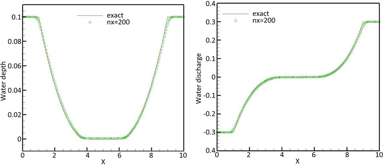
Figure 3. Water depth h (left) and water discharge hu (right) at t = 1
图3. t = 1时水深h (左)和水体动量hu (右)
4. 结论
本文设计了一种有效的保正高阶ADER-DG方法,用于求解具有非平坦底地形的一维浅水波方程。所提出的方法具有两个良好的特点:对静水稳态解具有良好的平衡性和在干湿锋附近保持正性。通过一种新颖的源项分裂和每个分裂源项的适当的良好平衡近似来实现良好平衡特性。采用 [63] 中的一个简单的保正限幅器,以确保所得方法保持截面湿面积的非负性。我们进行了相应的数值模拟实验,结果表明本文所提出的方法具有良好的平衡性,在稳态解附近的小扰动测试中有效,在干湿前沿附近保持正性以及高阶精度,并且在连续解和间断解上都表现良好。
基金项目
本研究得到了山东省自然科学基金面上项目(No. ZR2021MA072, ZR2023MA012)的资助。
文章引用
周翔宇,张志壮,钱守国,李 刚. 浅水波方程的高阶保正Well-Balanced ADER间断Galerkin格式
High Order Well-Balanced ADER Discontinuous Galerkin Scheme for Shallow Water Wave Equations[J]. 应用数学进展, 2023, 12(08): 3728-3743. https://doi.org/10.12677/AAM.2023.128367
参考文献
- 1. Vázquez-Cendón, M.E. (1999) Improved Treatment of Source Terms in Upwind Schemes for the Shallow Water Equa-tions in Channels with Irregular Geometry. Journal of Computational Physics, 148, 497-526. https://doi.org/10.1006/jcph.1998.6127
- 2. Garcia-Navarro, P. and Vázquez-Cendón, M.E. (2000) On Numerical Treatment of the Source Terms in the Shallow Water Equations. Computers & Fluids, 29, 951-979. https://doi.org/10.1016/S0045-7930(99)00038-9
- 3. Balbas, J. and Karni, S. (2009) A Central Scheme for Shal-low Water Flows along Channels with Irregular Geometry. ESAIM: Mathematical Modelling and Numerical Analysis, 43, 333-351. https://doi.org/10.1051/m2an:2008050
- 4. Hernández-Dueñas, G. and Karni, S. (2011) Shallow Water Flows in Channels. Journal of Scientific Computing, 48, 190-208. https://doi.org/10.1007/s10915-010-9430-x
- 5. Audusse, E., Bouchut, F., Bristeau, M.-O., Klein, R. and Per-thame, B. (2004) A Fast and Stable Well-Balanced Scheme with Hydrostatic Reconstruction for Shallow Water Flows. SIAM Journal on Scientific Computing, 25, 2050-2065. https://doi.org/10.1137/S1064827503431090
- 6. Xing, Y. and Shu, C.-W. (2005) High Order Finite Difference WENO Schemes with the Exact Conservation Property for the Shallow Water Equations. Journal of Computational Physics, 208, 206-227. https://doi.org/10.1016/j.jcp.2005.02.006
- 7. LeVeque, R.J. (1998) Balancing Source Terms and Flux Gradients in High-Resolution Godunov Methods: The Quasi-Steady Wave-Propagation Algorithm. Journal of Computational Physics, 146, 346-365. https://doi.org/10.1006/jcph.1998.6058
- 8. Perthame, B. and Simeoni, C. (2001) A Kinetic Scheme for the Saint-Venant System with a Source Term. Calcolo, 38, 201-231. https://doi.org/10.1007/s10092-001-8181-3
- 9. Xu, K. (2002) A Well-Balanced Gas-Kinetic Scheme for the Shallow-Water Equations with Source Terms. Journal of Computational Physics, 178, 533-562. https://doi.org/10.1006/jcph.2002.7040
- 10. Xing, Y. and Shu, C.-W. (2013) High Order Well-Balanced WENO Scheme for the Gas Dynamics Equations under Gravitational Fields. Journal of Scientific Computing, 54, 645-662. https://doi.org/10.1007/s10915-012-9585-8
- 11. Xing, Y. (2014) Exactly Well-Balanced Discontinuous Galerkin Methods for the Shallow Water Equations with Moving Water Equilibrium. Journal of Computational Physics, 257, 536-553. https://doi.org/10.1016/j.jcp.2013.10.010
- 12. Bermudez, A. and Vazquez, M.E. (1994) Upwind Meth-ods for Hyperbolic Conservation Laws with Source Terms. Computers & Fluids, 23, 1049-1071. https://doi.org/10.1016/0045-7930(94)90004-3
- 13. Xing, Y.L., Zhang, X.X. and Shu, C.-W. (2010) Positivi-ty-Preserving High Order Well-Balanced Discontinuous Galerkin Methods for the Shallow Water Equations. Advances in Water Resources, 33, 1476-1493. https://doi.org/10.1016/j.advwatres.2010.08.005
- 14. Bokhove, O. (2005) Flooding and Drying in Discontinuous Galerkin Finite-Element Discretizations of Shallow-Water Equations. Part 1: One Dimension. Journal of Scientific Com-puting, 22, 47-82. https://doi.org/10.1007/s10915-004-4136-6
- 15. Ern, A., Piperno, S. and Djadel, K. (2008) A Well-Balanced Runge-Kutta Discontinuous Galerkin Method for the Shallow-Water Equations with Flooding and Drying. International Journal for Numerical Methods in Fluids, 58, 1-25. https://doi.org/10.1002/fld.1674
- 16. Bunya, S., Kubatko, E.J., Westerink, J.J. and Dawson, C. (2009) A Wetting and Drying Treatment for the Runge-Kutta Discontinuous Galerkin Solution to the Shallow Water Equations. Computer Methods in Applied Mechanics and Engineering, 198, 1548-1562. https://doi.org/10.1016/j.cma.2009.01.008
- 17. Kurganov, A. and Levy, D. (2002) Central-Upwind Schemes for the Saint-Venant System. M2AN Mathematical Modelling and Numerical Analysis, 36, 397-425. https://doi.org/10.1051/m2an:2002019
- 18. Jiang, G.S. and Shu, C.W. (1996) Efficient Implementation of Weighted ENO Schemes. Journal of Computational Physics, 126, 202-212. https://doi.org/10.1006/jcph.1996.0130
- 19. Titarev, V.A. and Toro, E.F. (2002) ADER: Arbitrary High Order Godunov Approach. Journal of Scientific Computing, 17, 609-618. https://doi.org/10.1023/A:1015126814947
- 20. Titarev, V.A. and Toro, E.F. (2005) ADER Schemes for Three-Dimensional Non-Linear Hyperbolic Systems. Journal of Computational Physics, 204, 715-736. https://doi.org/10.1016/j.jcp.2004.10.028
- 21. Dumbser, M. and Munz, C.D. (2005) ADER Discontinuous Ga-lerkin Schemes for Aeroacoustics. Comptes Rendus Mécanique, 333, 683-687. https://doi.org/10.1016/j.crme.2005.07.008
- 22. Hu, C. and Shu, C.-W. (1999) Weighted Essentially Non-Oscillatory Schemes on Triangular Meshes. Journal of Computational Physics, 150, 97-127. https://doi.org/10.1006/jcph.1998.6165
- 23. Toro, E.F., Spruce, M. and Speares, W. (1994) Restoration of the Contact Surface in the HLL-Riemann Solver. Shock Waves, 4, 25-34. https://doi.org/10.1007/BF01414629
- 24. Zanotti, O., Fambri, F., Dumbser, M. and Hidalgo, A. (2015) Space-Time Adaptive ADER Discontinuous Galerkin Finite Element Schemes with a Posteriori Sub-Cell Finite Volume Limiting. Computers & Fluids, 118, 204-224. https://doi.org/10.1016/j.compfluid.2015.06.020
- 25. Fambri, F., Dumbser, M. and Zanotti, O. (2017) Space-Time Adaptive ADER-DG Schemes for Dissipative Flows: Compressible Navier-Stokes and Resistive MHD Equations. Computer Physics Communications, 220, 297-318. https://doi.org/10.1016/j.cpc.2017.08.001
- 26. Atkins, H.L. and Shu, C.-W. (1998) Quadrature-Free Implementa-tion of Discontinuous Galerkin Method for Hyperbolic Equations. AIAA Journal, 36, 775-782. https://doi.org/10.2514/2.436
- 27. Rannabauer, L., Dumbser, M. and Bader, M. (2018) ADER-DG with aPosterio-ri Finite-Volume Limiting to Simulate Tsunamis in a Parallel Adaptive Mesh Refinement Framework. Computers & Flu-ids, 173, 299-306. https://doi.org/10.1016/j.compfluid.2018.01.031
- 28. Harten, A. (1987) Uniformly High Order Accurate Essen-tially Non-oscillatory Schemes, III. Journal of Computational Physics, 71, 231-303. https://doi.org/10.1016/0021-9991(87)90031-3
- 29. Dumbser, M. and Munz, C.-D. (2006) Building Blocks for Arbitrary High Order Discontinuous Galerkin Schemes. Journal of Scientific Computing, 27, 215-230. https://doi.org/10.1007/s10915-005-9025-0
- 30. Dumbser, M., Hidalgo, A. and Zanotti, O. (2014) High Order Space-Time Adaptive ADER-WENO Finite Volume Schemes for Non-Conservative Hyperbolic Systems. Computer Methods in Applied Mechanics and Engineering, 268, 359-387. https://doi.org/10.1016/j.cma.2013.09.022
- 31. Duan, J. and Tang, H. (2020) An Efficient ADER Discontinuous Galerkin Scheme for Directly Solving Hamilton-Jacobi Equation. Journal of Computational Mathematics, 38, 58-83. https://doi.org/10.4208/jcm.1902-m2018-0189
- 32. Dumbser, M., Enaux, C. and Toro, E.F. (2008) Finite Volume Schemes of Very High Order of Accuracy for Stiff Hyperbolic Balance Laws. Journal of Computational Physics, 227, 3971-4001. https://doi.org/10.1016/j.jcp.2007.12.005
- 33. Courant, R., Isaacson, E. and Rees, M. (1952) On the Solution of Nonlinear Hyperbolic Differential Equations by Finite Differences. Communications on Pure and Applied Mathematics, 5, 243-255. https://doi.org/10.1002/cpa.3160050303
- 34. Shu, C.-W. (2016) High Order WENO and DG Methods for Time-Dependent Convection Dominated PDEs: A Brief Survey of Several Recent Developments. Journal of Computa-tional Physics, 316, 598-613. https://doi.org/10.1016/j.jcp.2016.04.030
- 35. Cockburn, B. and Shu, C.-W. (2001) Runge-Kutta Discontinuous Galerkin Methods for Convection Dominated Problems. Journal of Scientific Computing, 16, 173-261. https://doi.org/10.1023/A:1012873910884
- 36. Cockburn, B., Li, F. and Shu, C.-W. (2004) Locally Diver-gence-Free Discontinuous Galerkin Methods for the Maxwell Equations. Journal of Computational Physics, 194, 588-610. https://doi.org/10.1016/j.jcp.2003.09.007
- 37. Li, F. and Shu, C.-W. (2005) Locally Divergence-Free Discontinuous Galerkin Methods for MHD Equations. Journal of Scientific Computing, 22, 413-442. https://doi.org/10.1007/s10915-004-4146-4
- 38. Aizinger, V. and Dawson, C. (2002) A Discontinuous Galerkin Method for Two-Dimensional Flow and Transport in Shallow Water. Advances in Water Resources, 25, 67-84. https://doi.org/10.1016/S0309-1708(01)00019-7
- 39. Nair, R.D., Thomas, S.J. and Loft, R.D. (2005) A Discon-tinuous Galerkin Global Shallow Water Model. Monthly Weather Review, 133, 876-888. https://doi.org/10.1175/MWR2903.1
- 40. Schwanenberg, D. and Harms, M. (2004) Discontinuous Galerkin Fi-nite-Element Method for Tanscritical Two-Dimensional Shallow Water Flow. Journal of Hydraulic Engineering, 130, 412-421. https://doi.org/10.1061/(ASCE)0733-9429(2004)130:5(412)
- 41. Fagherazzi, S., Rasetarinera, P., Hussaini, Y.M. and Furbish, D.J. (2004) Numerical Solution of the Dam-Break Problem with a Discontinuous Galerkin Method. Journal of Hydraulic Engineering, 130, 532-539. https://doi.org/10.1061/(ASCE)0733-9429(2004)130:6(532)
- 42. Eskilsson, C. and Sherwin, S.J. (2004) A Trian-gular Spectral/hp Discontinuous Galerkin Method for Modelling 2D Shallow Water Equations. International Journal for Numerical Methods in Fluids, 45, 605-623. https://doi.org/10.1002/fld.709
- 43. Aureli, F., Maranzoni, A., Mignosa, P. and Ziveri, C.A. (2008) Weighted Sur-face-Depth Gradient Method for the Numerical Integration of the 2D Shallow Water Equations with Topography. Ad-vances in Water Resources, 31, 962-974. https://doi.org/10.1016/j.advwatres.2008.03.005
- 44. Canestrelli, A., Siviglia, A., Dumbser, M. and Toro, E.F. (2009) Well-Balanced High-Order Centred Schemes for Non-Conservative Hyperbolic Systems. Applications to Shallow Water Equations with Fixed and Mobile Bed. Advances in Water Resources, 32, 834-844. https://doi.org/10.1016/j.advwatres.2009.02.006
- 45. Kesserwani, G., Liang, Q., Vazquez, J. and Mose, R. (2010) Well-Balancing Issues Related to the RKDG2 Scheme for the Shallow Water Equations. International Journal for Nu-merical Methods in Fluids, 62, 428-448. https://doi.org/10.1002/fld.2027
- 46. Benkhaldoun, F., Elmahi, I. and Sead, M. (2010) A New Finite Volume Method for Flux-Gradient and Source-Term Balancing in Shallow Water Equations. Computer Methods in Applied Me-chanics and Engineering, 199, 3224-3335. https://doi.org/10.1016/j.cma.2010.07.003
- 47. Kesserwani, G. and Liang, Q.H. (2010) A Discontinuous Galerkin Algorithm for the Two-Dimensional Shallow Water Equations. Computer Methods in Applied Mechanics and Engineer-ing, 199, 3356-3368. https://doi.org/10.1016/j.cma.2010.07.007
- 48. Qian, S., Li, G., Shao, F. and Xing, Y. (2018) Positivity-Preserving Well-Balanced Discontinuous Galerkin Methods for the Shallow Water Flows in Open Channels. Advances in Water Resources, 115, 172-184. https://doi.org/10.1016/j.advwatres.2018.03.001
- 49. Chen, C.-K. and Ho, S.-H. (1996) Application of Differential Transformation to Eigenvalue Problems. Applied Mathematics and Computation, 79, 173-188. https://doi.org/10.1016/0096-3003(95)00253-7
- 50. Ayaz, F. (2003) On the Two-Dimensional Differential Trans-form Method. Applied Mathematics and Computation, 143, 361-374. https://doi.org/10.1016/S0096-3003(02)00368-5
- 51. Ayaz, F. (2004) Solutions of the System of Differential Equations by Differential Transform Method. Applied Mathematics and Computation, 147, 547-567. https://doi.org/10.1016/S0096-3003(02)00794-4
- 52. Kurnaza, A., Oturanç, G. and Kiris, M.E. (2005) n-Dimensional Differential Transformation Method for Solving PDEs. International Journal of Computer Mathematics, 82, 369-380. https://doi.org/10.1080/0020716042000301725
- 53. Norman, M.R. and Finkel, H. (2012) Mul-ti-Moment ADER-Taylor Methods for Systems of Conservation Laws with Source Terms in One Dimension. Journal of Computational Physics, 231, 6622-6642. https://doi.org/10.1016/j.jcp.2012.05.029
- 54. Zhang, X. and Shu, C.-W. (2010) On Maxi-mum-Principle-Satisfying High Order Schemes for Scalar Conservation Laws. Journal of Computational Physics, 229, 3091-3120. https://doi.org/10.1016/j.jcp.2009.12.030
- 55. Xing, Y. and Zhang, X. (2013) Positivity-Preserving Well-Balanced Discontinuous Galerkin Methods for the Shallow Water Equations on Unstructured Triangular Meshes. Journal of Computational Physics, 57, 19-41. https://doi.org/10.1007/s10915-013-9695-y
- 56. Xing, Y. (2016) High Order Finite Volume WENO Schemes for the Shallow Water Flows through Channels with Irregular Geometry. Journal of Computational and Applied Mathemat-ics, 299, 229-244. https://doi.org/10.1016/j.cam.2015.11.042
- 57. Liang, Q. and Marche, F. (2009) Numerical Resolution of Well-Balanced Shallow Water Equations with Complex Source Terms. Advances in Water Resources, 32, 873-884. https://doi.org/10.1016/j.advwatres.2009.02.010
- 58. Xing, Y. and Shu, C.-W. (2006) A New Approach of High Order Well-Balanced Finite Volume WENO Schemes and Discontinuous Galerkin Methods for a Class of Hyperbolic Systems with Source Terms. Computer Communications Physics, 1, 100-134.
- 59. Xing, Y. and Shu, C.-W. (2006) High Order Well-Balanced Finite Volume WENO Schemes and Discontinuous Galerkin Methods for a Class of Hyper-bolic Systems with Source Terms. Journal of Computational Physics, 214, 567-598. https://doi.org/10.1016/j.jcp.2005.10.005
- 60. Gallouen, T., Hérard, J.-M. and Seguin, N. (2003) Some Approxi-mate Godunov Schemes to Compute Shallow-Water Equations with Topography. Computers & Fluids, 32, 479-513. https://doi.org/10.1016/S0045-7930(02)00011-7
- 61. Xing, Y. and Shu, C.-W. (2011) High-Order Finite Volume WENO Schemes for the Shallow Water Equations with Dry States. Advances in Water Resources, 34, 1026-1038. https://doi.org/10.1016/j.advwatres.2011.05.008
- 62. Castro, M.J., Gallardo, J.M. and Parés, C. (2006) High Order Finite Volume Schemes Based on Reconstruction of States for Solving Hyperbolic Systems with Nonconservative Prod-ucts. Applicationssss to Shallow-Water Systems. Mathematics of Computation, 75, 1103-1134. https://doi.org/10.1090/S0025-5718-06-01851-5
- 63. Harten, A., Lax, P.D. and van Leer, B. (1983) On Upstream Differencing and Godunov-Type Schemes for Hyperbolic Conservation Laws. Society for Industrial and Applied Math-ematics Review, 25, 35-61. https://doi.org/10.1137/1025002