基于Gronwall积分不等式的Hopfield神经网络稳定性的新判据 A New Criterion for Stability of Hopfield Neural Network Based on Gronwall Integral Inequality

doi:10.12677/AAM.2018.712194

Advances in Applied Mathematics
Vol. 07 No. 12 ( 2018 ), Article ID: 28302 , 9 pages
10.12677/AAM.2018.712194

A New Criterion for Stability of Hopfield Neural Network Based on Gronwall Integral Inequality

Xingshou Huang, Ricai Luo, Wusheng Wang

●How to Cite this Article

School of Mathematics and Statistics, Hechi University, Yizhou Guangxi

Received: Dec. 2^nd, 2018; accepted: Dec. 22^nd, 2018; published: Dec. 29^th, 2018

ABSTRACT

When people study Hopfield time-delay neural network, Lyapunov function is usually used to analyze the stability of the system. But, in this paper, we study the stability of Hopfield neural network by using Gronwall integral inequalities, and obtain the new criterion of global exponential stability of Hopfield neural network and its delay system. Finally, we demonstrate the validity of the results by a numerical example.

Keywords:Gronwall Integral Inequalities, Hopfield Neural Networks, Time Delays, Exponential Stability

基于Gronwall积分不等式的Hopfield神经网络稳定性的新判据

黄星寿，罗日才，王五生

河池学院，数学与统计学院，广西宜州

收稿日期：2018年12月2日；录用日期：2018年12月22日；发布日期：2018年12月29日

摘要

在Hopfield时滞神经网络的研究中，人们通常是利用构造李亚普诺夫函数来分析系统的稳定性。本文利用一类Gronwall积分不等式研究了Hopfield神经网络的稳定性问题，我们得出Hopfield神经网络及其时滞系统全局指数稳定性的新判据，并通过实例仿真验证了结果的有效性和可行性。

关键词 :Gronwall积分不等式，Hopfield神经网络，时滞，指数稳定性

This work is licensed under the Creative Commons Attribution International License (CC BY).

http://creativecommons.org/licenses/by/4.0/

1. 引言

自从Hopfield [1] 在1984年提出他名字命名的Hopfield神经网络以来，这类人工神经网络在很多方面得到了广泛的应用，如组合优化 [2] [3] [4] ，图像处理 [5] [6] ，模式识别 [7] ，信号处理 [8] ，通讯技术 [9] 等等，所以在过去的数十年中，Hopfield神经网络被持续研究 [10] - [23] 。由于在神经网络的实际应用中，一方面由于两个神经元之间信息传递不免存在时滞，另一方面由于受到诸如有限的开关速度等硬件的影响，时滞现象也是不可避免的，在神经网络研究中引入时滞得到了广泛的关注 [15] - [22] 。

人们在Hopfield神经网络的研究中所采用的方法通常是利用构造李亚普诺夫函数并结合线性矩阵不等式来分析系统的稳定性。无疑，李亚普诺夫方法是微分方程稳定性研究的利器，但是如何构造适当的李亚普诺夫是解决问题的关键，也是一个难题，另外，同一个系统，构造不同的李亚普诺夫函数，得到的稳定性范围也可能不相同，而且线性矩阵不等式的运算也很繁琐。

Gronwall不等式在微分方程定性理论研究中也发挥极其重要的作用，并且得到不断的推广和广泛应用 [23] - [38] ，但是用于研究神经网络系统的稳定性比较少见。

本文利用Gronwall积分不等式研究对如下对Hopfield时滞神经网络模型的稳定性问题。

$\dot{x} (t) = - A x (t) + B g (x (t)) + C g (x (t - τ)) + I$ (1)

其中 $x (t) = {(x_{1} (t), x_{2} (t), \dots, x_{n} (t))}^{T}$ 表示神经元的状态变量， $g (x (t)) = (g_{1} (x_{1} (t)), g_{2} (x_{2} (t)), \dots, g_{n} (x_{n} (t)))$ 表示激活函数， $g (x (t - τ))$ 为时滞项激活函数， $A = d i a g {a_{1}, a_{2}, \dots, a_{n}}$ ( $a_{i} > 0, i = 1, 2, \dots, n$ )， $B = {(b_{i j})}_{n \times n}$ ， $C = {(c_{i j})}_{n \times n}$ ，分别表示对应神经元的连接权重系数矩阵，其中，a_i表示第i个神经元的自反馈强度， $b_{i j}$ 表示第j个神经元的输出 $g_{j} (x_{j} (t))$ 对于第i个神经元的输入的反馈连接强度，如果第j个神经元的输出使第i个神经元激活(或抑制)，则 $b_{i j} > 0$ (或 $b_{i j} < 0$ )； $c_{i j}$ 类似。τ表示传输时滞，为某一正常数。

这里我们定义n × n矩阵 $M = {(a_{i j})}_{n \times n}$ 和n维向量 $x = {(x_{1}, x_{2}, \dots, x_{n})}^{T}$ 的范数为：

$‖ M ‖ = \sqrt{λ_{\max} (A^{T} A)}$ ，其中， $λ_{\max} (A^{T} A)$ 表示 $A^{T} A$ 的最大特征值， $‖ x ‖ = \sqrt{x_{1}^{2} + x_{2}^{2} + \dots + x_{n}^{2}}$ 。

我们假设激活函数f满足李普希兹条件： $‖ f (y) - f (x) ‖ \leq L ‖ y - x ‖$ 。

由于系统(2)的激活函数f满足李普希兹条件，所以存在唯一平衡点，这在很多文献已经做了证明 [15] - [20] ，这里不再重复。令系统(2)的平衡点为x^*，设 $y (t) = x (t) - x^{*}$ 。那么系统(2)可变为

$\dot{y} (t) = - A y (t) + B f (y (t)) + C f (y (t - τ))$ , (2)

其中， $f (y) = g (y + x^{*}) - g (x^{*})$ ，其它各个符号的含义与系统(1)相同。

引理(Gronwall不等式) [24] ：设K为非负常数，u(t)和g(t)为在区间 $α \leq t \leq β$ 上的非负连续函数，且满足不等式

$u (t) \leq K + \int_{α}^{t} u (s) g (s) d s, α \leq t \leq β$

则有

$u (t) \leq K \cdot \exp [\int_{α}^{t} g (s) d s], α \leq t \leq β$ .

2. 稳定性分析

2.1. 无时滞的情形分析

考虑系统

$\dot{y} (t) = - A y (t) + B f (y (t))$ (3)

系统(3)的线性系统为

$\dot{y} (t) = - A y (t)$ (4)

基解矩阵为

$\exp [- A t] = [\begin{matrix} e^{- a_{1} t} & 0 \\ e^{- a_{2} t} \\ ⋱ \\ 0 & e^{- a_{n} t} \end{matrix}]$ ,

设初值 $t = 0$ 时，对应初值为 $η = (η_{1}, η_{2}, \dots, η_{n})$ ，那么系统(4)的解可以表示为 $Y (t) = (η_{1} e^{- a_{1} t}, η_{2} e^{- a_{2} t}, \dots, η_{n} e^{- a_{n} t})$ ，取范数 $‖ Y (t) ‖ = \sqrt{{(| η_{1} | e^{- a_{1} t})}^{2} + {(| η_{2} | e^{- a_{2} t})}^{2} + \dots + {(| η_{n} | e^{- a_{n} t})}^{2}}$ ，做以下记号：

I) $M = \sqrt{n} \cdot \max {| η_{1} |, | η_{2} |, \dots, | η_{n} |}$ ，显然，M > 0。

II) $σ = \min {a_{1}, a_{2}, \dots, a_{n}}$ 。

可得 $‖ Y (t) ‖ \leq M e^{- σ t}$ 。

定理1：激活函数 $f (y (t))$ 满足利普希茨条件下，当 $L ‖ B ‖ - σ < 0$ 时，系统(3)的零解是全局指数稳定的。

证明：设Y(t)为方程(4)的解，由常数变易法得方程(3)的解可以表示为

$y (t) = Y (t) + \int_{0}^{t} e^{- A (t - s)} B f (y (s)) d s$ ，实际上，这里 $Y (t) = e^{- A t} η$ ，两边取范数

$\begin{matrix} ‖ y (t) ‖ = ‖ Y (t) ‖ + \int_{0}^{t} ‖ e^{- A (t - s)} B f (y (s)) ‖ d s \\ \leq M e^{- σ t} + \int_{0}^{t} ‖ e^{- A (t - s)} ‖ ‖ B ‖ ‖ f (y (s)) ‖ d s \\ \leq M e^{- σ t} + L ‖ B ‖ \int_{0}^{t} e^{- σ (t - s)} ‖ y (s) ‖ d s \end{matrix}$

两边同时乘以 $e^{σ t}$ ，可得

$e^{σ t} ‖ y (t) ‖ \leq M + L ‖ B ‖ \int_{0}^{t} e^{σ s} ‖ y (s) ‖ d s$

根据引理1 (Gronwall不等式)得

$e^{σ t} ‖ y (t) ‖ \leq M e^{L ‖ B ‖ \int_{0}^{t} d s} = M e^{L ‖ B ‖ t}$

两边同时除以 $e^{σ t}$ ，得 $‖ y (t) ‖ \leq M e^{(L ‖ B ‖ - σ) t}$ ，由已知条件 $L ‖ B ‖ - σ < 0$ ，可得系统(3)的零解是全局指数稳定的。定理得证。

2.2. 具有时滞的情况分析

设

$D (y) = [\begin{matrix} f_{1} (y_{1}) / y_{1} & 0 \\ f_{2} (y_{2}) / y_{2} \\ ⋱ \\ 0 & f_{n} (y_{n}) / y_{n} \end{matrix}]$ (5)

系统(3)可以表示为

$\dot{y} (t) = (- A + B D (y)) y (t)$ (6)

设初值 $t = 0$ 时，对应初值为 $η = (η_{1}, η_{2}, \dots, η_{n})$ ，系统(6)的解为向量函数 $φ (t)$ ，设 $σ - L ‖ B ‖ = σ_{1}$ (>0)那么由定理1可得

$‖ φ (t) ‖ \leq ‖ η ‖ e^{- σ_{1} t}$ (7)

定理2：激活函数 $f (\cdot)$ 满足利普希茨条件下，当 $e^{σ_{1} τ} ‖ C ‖ L - σ_{1} < 0$ 时，系统(2)是全局指数稳定的。

证明：由(5)式，系统(2)改写为

$\dot{y} (t) = (- A + B D (y)) y (t) + C f (y (t - τ))$ (8)

当 $t = 0$ 时，对应初值为 $η = (η_{1}, η_{2}, \dots, η_{n})$ ，方程(8)的解可以表示为

$y (t) = φ (t) + \int_{0}^{t} e^{(L ‖ B ‖ E - A) (t - s)} C f (y (s - τ)) d s$

两边取范数，有

$\begin{matrix} ‖ y (t) ‖ \leq ‖ φ (t) ‖ + \int_{0}^{t} ‖ e^{(L ‖ B ‖ E - A) (t - s)} C f (y (s - τ)) ‖ d s \\ \leq ‖ φ (t) ‖ + \int_{0}^{t} ‖ e^{(L ‖ B ‖ E - A) (t - s)} ‖ ‖ C ‖ ‖ f (y (s - τ)) ‖ d s \\ \leq ‖ η ‖ e^{- σ_{1} t} + \int_{- τ}^{t - τ} e^{(L ‖ B ‖ - σ) (t - τ - s)} ‖ C ‖ L ‖ y (s) ‖ d s \\ = ‖ η ‖ e^{- σ_{1} t} + e^{σ_{1} t} ‖ C ‖ L \int_{- τ}^{t - τ} e^{- σ_{1} (t - s)} ‖ y (s) ‖ d s \end{matrix}$

两边同时乘以 $e^{σ_{1} t}$ ，可得

$\begin{matrix} e^{σ_{1} t} ‖ y (t) ‖ = ‖ η ‖ + e^{σ_{1} t} ‖ C ‖ L \int_{- τ}^{t - τ} e^{σ_{1} t} e^{- σ_{1} (t - s)} ‖ y (s) ‖ d s \\ = ‖ η ‖ + e^{σ_{1} t} ‖ C ‖ L \int_{- τ}^{t - τ} e^{σ_{1} s} ‖ y (s) ‖ d s \end{matrix}$

根据引理1 (Gronwall不等式)得

$e^{σ_{1} t} ‖ y (t) ‖ \leq ‖ η ‖ e^{e^{σ_{1} τ} ‖ C ‖ L \int_{- τ}^{t - τ} d s} = ‖ η ‖ e^{e^{σ_{1} τ} ‖ C ‖ L t}$

所以 $‖ y (t) ‖ \leq ‖ η ‖ e^{e^{σ_{1} τ} ‖ C ‖ L \int_{- τ}^{t - τ} d s} e^{- σ_{1} t} = ‖ η ‖ e^{(e^{σ_{1} τ} ‖ C ‖ L - σ_{1}) t}$ ，由于 $e^{σ_{1} τ} ‖ C ‖ L - σ_{1} < 0$ ，所以系统(8)即时滞系统(2)是全局指数稳定的。

3. 数值仿真

这一节，我们用一个实际例子来验证定理结果的有效性。

例1：考虑如下无时滞二维神经网络模型：

$(\begin{matrix} \dot{x} (t) \\ \dot{y} (t) \end{matrix}) = - A (\begin{matrix} x (t) \\ y (t) \end{matrix}) + B (\begin{matrix} f_{1} (x (t)) \\ f_{2} (y (t)) \end{matrix})$ (9)

其中，激活函数 $f_{i} (u) = \frac{e^{u} - 1}{e^{u} + 1}$ ， $i = 1, 2$ ，显然满足李普希兹条件，并且 $L = 0. 5$ ，

显然，如果我们取 $A = [\begin{matrix} 1 & 0 \\ 0 & 1 \end{matrix}]$ ， $B = [\begin{matrix} 0.9 & 0.8 \\ 0.4 & - 0.5 \end{matrix}]$ ，那么， $σ = 1$ ， $‖ B ‖ = 1.3$ ， $L ‖ B ‖ - σ = - 0.35$ ，当 $t = 0$ 时，初值取 $(x (0), y (0)) = (10, 10)$ ，状态轨线图如图1所示，系统(9)的零解是指数稳定的。

Figure 1. The state rail diagram of system (9) ( $L ‖ B ‖ - σ < 0$ )

图1. 系统(9)的状态轨线图( $L ‖ B ‖ - σ < 0$ )

如果我们取 $A = [\begin{matrix} 2 & 0 \\ 0 & 2 \end{matrix}]$ ， $B = [\begin{matrix} 10 & - 20 \\ 25 & - 10 \end{matrix}]$ ，那么 $σ = 2$ ， $‖ B ‖ = 35$ ， $L ‖ B ‖ - σ = 15.5$ ，当 $t = 0$ 时，初值取 $(x (0), y (0)) = (10, 10)$ ，状态轨线图如图2所示，此时系统(9)是稳定的，但不是指数稳定的。

例2：考虑如下无时滞二维神经网络模型：

$(\begin{matrix} \dot{x} (t) \\ \dot{y} (t) \end{matrix}) = - A (\begin{matrix} x (t) \\ y (t) \end{matrix}) + B (\begin{matrix} f_{1} (x (t)) \\ f_{2} (y (t)) \end{matrix}) + C (\begin{matrix} f_{1} (x (t - τ)) \\ f_{2} (y (t - τ)) \end{matrix})$ (10)

其中，激活函数 $f_{i} (u) = \frac{e^{u} - 1}{e^{u} + 1}$ ， $i = 1, 2$ ，显然满足李普希兹条件，并且 $L = 0. 5$ ，

如果我们取 $A = [\begin{matrix} 1 & 0 \\ 0 & 1 \end{matrix}]$ ， $B = [\begin{matrix} 0.3 & 0.8 \\ 0.2 & - 0.5 \end{matrix}]$ ， $C = [\begin{matrix} 0.1 & - 0.3 \\ 0.2 & 0.5 \end{matrix}]$ ，时滞 $τ = 0. 5$ ，那么， $σ = 1$ ， $‖ B ‖ = 0.9565$ ， $‖ C ‖ = 0.5966$ ， $σ_{1} = σ - L ‖ B ‖ = 0.5217$ ， $e^{σ_{1} τ} ‖ C ‖ L - σ_{1} = - 0.1344 < 0$ ，根据定理2，系统(10)的零解是指数稳定的，当 $t = 0$ 时，初值取 $(x (0), y (0)) = (- 10, 10)$ ，系统状态轨线图如图3所示。

Figure 2. The state rail diagram of system (9) ( $L ‖ B ‖ - σ > 0$ )

图2. 系统(9)的状态轨线图( $L ‖ B ‖ - σ > 0$ )

Figure 3. The state rail diagram of system (10) ( $e^{σ_{1} τ} ‖ C ‖ L - σ_{1} < 0$ )

图3. 系统(10)的状态轨线图( $e^{σ_{1} τ} ‖ C ‖ L - σ_{1} < 0$ )

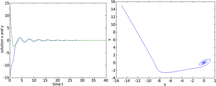
Figure 4. The state rail diagram of system (10) ( $e^{σ_{1} τ} ‖ C ‖ L - σ_{1} > 0$ )

图4. 系统(10)的状态轨线图( $e^{σ_{1} τ} ‖ C ‖ L - σ_{1} > 0$ )

如果我们取 $A = [\begin{matrix} 1 & 0 \\ 0 & 1 \end{matrix}]$ ， $B = [\begin{matrix} 0.3 & 0.8 \\ 0.2 & - 0.5 \end{matrix}]$ ， $C = [\begin{matrix} 1 & - 5 \\ 4 & - 4 \end{matrix}]$ ，时滞 $τ = 0.5$ ，那么， $σ = 1$ ， $‖ B ‖ = 0.9565$ ， $‖ C ‖ = 7.2929$ ， $σ_{1} = σ - L ‖ B ‖ = 0.5217$ ， $e^{σ_{1} τ} ‖ C ‖ L - σ_{1} = 4.2115 > 0$ ，当 $t = 0$ 时，初值取 $(x (0), y (0)) = (- 15, 15)$ ，系统的状态轨线图如图4，显然此时系统(10)是稳定的，但不是指数稳定的。

基金项目

广西自然科学基金项目(2016GXNSFAA380125, 2016GXNSFAA380090)。

文章引用

黄星寿,罗日才,王五生. 基于Gronwall积分不等式的Hopfield神经网络稳定性的新判据
A New Criterion for Stability of Hopfield Neural Network Based on Gronwall Integral Inequality[J]. 应用数学进展, 2018, 07(12): 1658-1666. https://doi.org/10.12677/AAM.2018.712194

参考文献

1. Hopfield, J.J. (1984) Neurons with Graded Response Have Collective Computational Properties Like Those of Two-State Neurons. Proceedings of the National Academy of Sciences of the USA, 81, 3088-3092. https://doi.org/10.1073/pnas.81.10.3088

2. Abe, S., Kawakami, J. and Hirasawa, K. (1992) Solving Inequality Constrained Combinatorial Optimization Problems by the Hopfield Neural Networks. Neural Networks, 5, 663-670. https://doi.org/10.1016/S0893-6080(05)80043-7

3. Tamura, H., Zhang, Z., Xu, X.S., Ishii, M. and Tang, Z. (2005) Lagrangian Object Relaxation Neural Network for Combinatorial Optimization Problems. Neurocomputing, 68, 297-305. https://doi.org/10.1016/j.neucom.2005.03.003

4. Wang, R.L., Tang, Z. and Cao, Q.P. (2002) A Learning Method in Hopfield Neural Network for Combinatorial Optimization Problem. Neurocomputing, 48, 1021-1024. https://doi.org/10.1016/S0925-2312(02)00596-9

5. Rout, S., Seethalakshmy, Srivastava, P. and Majumdar, J. (1998) Multi-Modal Image Segmentation Using a Modified Hopfield Neural Network Original Research Article. Pattern Recognition, 31, 743-750. https://doi.org/10.1016/S0031-3203(97)00089-7

6. Sammouda, R., Adgaba, N., Touir, A. and Al-Ghamdi, A. (2014) Agriculture Satellite Image Segmentation Using a Modified Artificial Hopfield Neural Network Original Research Article. Computers in Human Behavior, 30, 436-441. https://doi.org/10.1016/j.chb.2013.06.025

7. Suganthan, P., Teoh, E. and Mital, D. (1995) Pattern Recognition by Homomorphic Graph Matching Using Hopfield Neural Networks Original Research Article. Image and Vision Computing, 13, 45-60. https://doi.org/10.1016/0262-8856(95)91467-R

8. Laskaris, N., Fotopoulos, S., Papathanasopoulos, P. and Bezerianos, A. (1997) Robust Moving Averages, with Hopfield Neural Network Implementation, for Monitoring Evoked Potential Signals Original Research Article. Electroencephalography and Clinical Neurophysiology/Evoked Potentials Section, 104, 151-156.

9. Calabuig, D., Monserrat, J.F., Gmez-Barquero, D. and Lzaro, O. (2008) An Efficient Dynamic Resource Allocation Algorithm for Packet-Switched Communication Networks Based on Hopfield Neural Excitation Method Original Research Article. Neurocomputing, 71, 3439-3446. https://doi.org/10.1016/j.neucom.2007.10.009

10. Marcus, C. and Westervelt, R. (1989) Stability of Analog Neural Networks with Delay. Physical Review A, 39, 347-359. https://doi.org/10.1103/PhysRevA.39.347

11. Wu, J. (1999) Symmetric Functional-Differential Equations and Neural Networks with Memory. Transactions of the American Mathematical Society, 350, 4799-4838. https://doi.org/10.1090/S0002-9947-98-02083-2

12. Wu, J. and Zou, X. (1995) Patterns of Sustained Oscillations in Neural Networks with Time Delayed Interactions. Applied Mathematics and Computation, 73, 55-75.

13. Gopalsamy, K. and He, X. (1994) Stability in Asymmetric Hopfield Nets with Transmission Delays. Physica D, 76, 344-358. https://doi.org/10.1016/0167-2789(94)90043-4

14. Zhang, W.N. (2006) A Weak Condition of Globally Asymptotic Stability for Neural Networks. Applied Mathematics Letters, 19, 1210-1215. https://doi.org/10.1016/j.aml.2006.01.009

15. Orman, Z. (2012) New Sufficient Conditions for Global Stability of Neutral-Type Neural Networks with Time Delays. Neurocomputing, 97, 141-148. https://doi.org/10.1016/j.neucom.2012.05.016

16. Zhang, F. (2005) The Schur Complement and Its Applications. Numerical Methods and Algorithms, Vol. 4, Springer-Verlag, New York, 34.

17. Chen, Y. and Xu, H. (2012) Expo-nential Stability Analysis and Impulsive Tracking Control of Uncertain Time-Delayed Systems. Journal of Global Opti-mization, 52, 323-334. https://doi.org/10.1007/s10898-011-9669-2

18. Xu, H., Chen, Y. and Teo, K.L. (2010) Global Exponential Stability of Impulsive Discrete-Time Neural Networks with Time-Varying Delays. Applied Math-ematics and Computations, 217, 537-544. https://doi.org/10.1016/j.amc.2010.05.087

19. Forti, M. (1994) On Global Asymptotic Stability of a Class of Nonlinear Systems Arising in Neural Network Theory. Journal of Differential Equations, 113, 246-264. https://doi.org/10.1006/jdeq.1994.1123

20. Forti, M., Maneti, S. and Marini, M. (1994) Necessary and Sufficient Conditions for Absolute Stability of Neural Networks. IEEE Transactions on Circuits and Systems I, 41, 491-494. https://doi.org/10.1109/81.298364

21. Forti, M. and Tesi, A. (1995) New Conditions for Global Stability of Neural Networks with Application to Linear and Quadratic Programming Problems. IEEE Transactions on Circuits and Systems I, 42, 354-366. https://doi.org/10.1109/81.401145

22. Gasull, A., Llibre, J. and Sotomayor, J. (1991) Global Asymptotic Stability of Differential Equations in the Plane. Journal of Differential Equations, 91, 327-336. https://doi.org/10.1016/0022-0396(91)90143-W

23. Gronwall, T.H. (1919) Note on the Derivatives with Respect to a Parameter of the Solutions of a System of Differential Equations. Annals of Mathematics, 20, 292-296. https://doi.org/10.2307/1967124

24. Bellman, R. (1943) The Stability of Solutions of Linear Differential Equations. Duke Mathematical Journal, 10, 643-647. https://doi.org/10.1215/S0012-7094-43-01059-2

25. Abdeldaim, A. (2016) Nonlinear Retarded Integral Inequalities of Type and Applications. Journal of Mathematical Inequalities, 10, 285-299.

26. Lipovan, O. (2000) A Retarded Gronwall-Like Inequality and Its Applications. Journal of Mathematical Analysis and Applications, 252, 389-401. https://doi.org/10.1006/jmaa.2000.7085

27. Agarwal, R.P., Deng, S. and Zhang, W. (2005) Generalization of a Retarded Gronwall-Like Inequality and Its Applications. Applied Mathematics and Computation, 165, 599-612. https://doi.org/10.1016/j.amc.2004.04.067

28. Cheung, W.S. (2006) Some New Nonlinear Inequalities and Applications to Boundary Value Problems. Nonlinear Analysis, 64, 2112-2128. https://doi.org/10.1016/j.na.2005.08.009

29. Abdeldaim, A. and Yakout, M. (2011) On Some New Integral Ine-qualities of Gronwall-Bellman-Pachpatte Type. Applied Mathematics and Computation, 217, 7887-7899. https://doi.org/10.1016/j.amc.2011.02.093

30. El-Owaidy, H., Ragab, A.A., Abuelela, W. and El-Deeb, A.A. (2014) On Some New Nonlinear Integral Inequalities of Gronwall-Bellman Type. Kyungpook Mathematical Journal, 54, 555-575. https://doi.org/10.5666/KMJ.2014.54.4.555

31. Sano, H. and Kunimatsu, N. (1994) Modified Gronwall’s Inequality and Its Application to Stabilization Problem for Semilinear Parabolic Systems. Systems & Control Letters, 22, 145-156. https://doi.org/10.1016/0167-6911(94)90109-0

32. Ye, H.P., Gao, J.M. and Ding, Y.S. (2007) A Generalized Gronwall Inequality and Its Application to a Fractional Differential Equation. Journal of Math-ematical Analysis and Applications, 328, 1075-1081. https://doi.org/10.1016/j.jmaa.2006.05.061

33. Medved, M. (2002) Integral Inequalities and Global Solutions of Semilinear Evolution Equations. Journal of Mathematical Analysis and Applications, 267, 643-650. https://doi.org/10.1006/jmaa.2001.7798

34. Ma, Q.H. and Pecaric, J. (2008) Some New Explicit Bounds for Weakly Singular Integral Inequalities with Applications to Fractional Differential and Integral Equations. Journal of Mathematical Analysis and Applications, 341, 894-905. https://doi.org/10.1016/j.jmaa.2007.10.036

35. Deng, S. and Prather, C. (2008) Generalization of an Impulsive Nonlinear Singular Gronwall-Bihari Inequality with Delay. Journal of Inequalities in Pure and Applied Mathematics, 9, Article 34.

36. Mazouzi, S. and Tatar, N. (2010) New Bounds for Solutions of a Singular Integro-Differential Inequality. Mathematical Inequalities & Applications, 13, 427-435.

37. Wang, H. and Zheng, K. (2010) Some Nonlinear Weakly Singular Integral Inequalities with Two Vari-ables and Applications. Journal of Inequalities and Applications, 2010, Article ID: 345701.

38. Cheng, K., Guo, C. and Tang, M. (2014) Some Nonlinear Gronwall-Bellman-Gamidov Integral Inequalities and Their Weakly Singular Analogues with Applications. Abstract and Applied Analysis, 2014, Article ID: 562691.

期刊菜单