半直线上Kortewego-de Vries方程的Laguerre谱配置方法 Generalized Laguerre Spectral-Collocation Method for KdV Equations on the Half Line

doi:10.12677/AAM.2020.99186

Advances in Applied Mathematics
Vol. 09 No. 09 ( 2020 ), Article ID: 37789 , 6 pages
10.12677/AAM.2020.99186

半直线上Kortewego-de Vries方程的Laguerre谱配置方法

王其霞，苗伊浩，王天军

●How to Cite this Article

河南科技大学数学与统计学院，河南洛阳

收稿日期：2020年9月1日；录用日期：2020年9月17日；发布日期：2020年9月24日

摘要

以Laguerre-Gauss-Radau节点为配置点，用带松弛因子的Lagrange插值函数逼近半直线上的Kortewego-de Vries方程初边值问题的理论解，给出算法格式和相应的数值结果，表明所提算法格式的有效性和高精度。对理论解中参数的不同取值，通过适当地选择插值函数中的松弛因子，数值解可以很好地匹配理论解，而且所给算法对长时间的计算仍然有效。

关键词

Kortewego-de Vries方程初边值问题，Laguerre函数谱配置方法，Laguerre-Gauss-Radau节点，半直线

Generalized Laguerre Spectral-Collocation Method for KdV Equations on the Half Line

Qixia Wang, Yihao Miao, Tianjun Wang

College of Mathematics & Statistics, Henan University of Science & Technology, Luoyang Henan

Received: Sep. 1^st, 2020; accepted: Sep. 17^th, 2020; published: Sep. 24^th, 2020

ABSTRACT

Interpolation function approximations with relaxation factor by using Laguerre-Gauss-Radau nodes as collocation points to the Korteweg-de Vries equation on semi-infinite intervals are considered. The validity and high accuracy of the proposed algorithm are demonstrated. By choosing the relaxation factor of the interpolation function properly, the numerical solution can match the theoretical solution well, and the algorithm is still valid for a long time.

Keywords:Initial-Boundary Value Problem of Kortewego-de Vries Equations, Spectral Collocation Method of Laguerre Functions, Laguerre-Gauss-Radau Nodes, The Half Line

This work is licensed under the Creative Commons Attribution International License (CC BY 4.0).

http://creativecommons.org/licenses/by/4.0/

1. 引言

记 $R^{+} = {x | 0 < x < \infty}$ 为简单，记 $\frac{\partial u}{\partial z} = \partial_{z} u$ 。下式为半直线上Kortewego-de Vries (KdV)方程初边值

问题 [1] [2] [3]：

${\begin{cases} \partial_{t} u + γ u \partial_{x} u + ν \partial_{x}^{3} u = 0, x \in R^{+}, t > 0, \\ u (x, t), \partial_{x} u (x, t) \to 0, x \to + \infty, t \geq 0, \\ u (x, 0) = g_{0} (x), x \in R^{+}, \\ u (0, t) = g_{1} (t), t \geq 0. \end{cases}$ (1)

其中 $γ$ 和 $ν$ 是常数。文献 [4] [5] [6] 用谱方法或有限元/b-样条有限元方法研究有界区域上KdV方程的数值解，针对方程(1)中的参数 $γ, ν$ 的不同取值，文献 [7] [8] 利用空间Hermite谱配置方法、时间有限差分方法或Chebyshev-Hermite多项式时空谱配置方法求解其Cauchy问题的数值解；文献 [9] 用Laguerre拟谱方法研究了半直线上非线性热传导方程的数值解。针对问题(1)的孤波解的性态，用含有因子 $e^{- β x / 2} (β > 0)$ 的插值函数可以更好地逼近问题的理论解，同时通过适当选取伸缩因子 $β$ 可以改进数值误差精度。另外，用Gauss型节点得到的Lagrang插值多项式，与其相关的高阶微分矩阵是一阶微分矩阵的乘积，这为实际计算带来极大的方便。

2. 基于Gauss型节点的Lagrange插值函数及其微分矩阵

次数为l的广义拉盖尔多项式定义为 [9]：

$L_{l}^{(α, β)} (x) = \frac{1}{l!} x^{- α} e^{β x} \partial_{x}^{l} (x^{l + α} e^{- β x}), l = 0, 1, \dots .$ (2)

广义拉盖尔函数定义为：

${\tilde{L}}_{l}^{(α, β)} (x) = e^{- \frac{1}{2} β x} L_{l}^{(α, β)} (x), l = 0, 1, \dots .$ (3)

特别， $L_{l}^{(β)} (x) = L_{l}^{(0, β)} (x), {\tilde{L}}_{l}^{(β)} (x) = e^{- \frac{1}{2} β x} L_{l}^{(β)} (x)$ 。

令 $x_{j} (0 \leq j \leq N)$ 是 $x \partial_{x} L_{N + 1}^{(β)} (x) = 0$ 的根。以 $x_{j}$ 为节点的通常的Lagrange插值基函数为 [9] [10] [11]

$φ_{j}^{(β)} (x) = \frac{e^{- β x / 2}}{β (N + 1) e^{- β x_{j} / 2}} \frac{x \partial_{x} L_{N + 1}^{(β)} (x)}{(x_{j} - x) L_{N + 1}^{(β)} (x_{j})}, j = 0, 1, \dots, N$

对任意 $u (x) \in C (R^{+})$ ，其Lagrange插值多项式为：

$p_{N}^{(β)} (x) = \sum_{j = 0}^{N} u (x_{j}) φ_{j}^{(β)} (x), x \in R^{+} .$

对 $p_{N} (x)$ 求m阶导数得，

$\partial_{x}^{m} p_{N}^{(β)} (x) = \sum_{j = 0}^{N} u (x_{j}) \partial_{x}^{m} φ_{j}^{(β)} (x) .$

令

$D^{(m)} = {(\partial_{x}^{m} φ_{j}^{(β)} (x_{k}))}_{0 \leq k, j \leq N}, D : = D^{(1)} = (d_{k, j}^{(β)} = \partial_{x} φ_{j}^{(β)} (x_{k})),$

则由文献 [9] [10] [11]

$d_{k, j}^{(β)} = {\begin{cases} \frac{{\tilde{L}}_{N + 1}^{(β)} (x_{k})}{(x_{k} - x_{j}) {\tilde{L}}_{N + 1}^{(β)} (x_{j})}, k \neq j, \\ - \frac{(N + 1) β}{2}, k = j = 0, \\ 0, k = j \neq 0. \end{cases}$ (4)

$D^{(m)} = D^{m} .$ (5)

特别，

$D^{(3)} = {({\tilde{d}}_{k, j}^{(β)} = \partial_{x}^{3} φ_{j}^{(β)} (x_{k}))}_{0 \leq k, j \leq N} .$

3. KdV方程的谱配置方法

3.1. KdV方程的谱配置格式

在式(1)中去 $γ = ν = 1$ ，考虑KdV方程的初边值问题：

${\begin{cases} \partial_{t} u + u \partial_{x} u + \partial_{x}^{3} u = 0, x \in R^{+}, t > 0, \\ u (x, t), \partial_{x} u (x, t) \to 0, x \to + \infty, t \geq 0, \\ u (x, 0) = g_{0} (x), x \in R^{+}, \\ u (0, t) = g_{1} (t), t \geq 0. \end{cases}$ (6)

用 $w_{N} (x, t) = \sum_{j = 0}^{N} u (x_{j}, t) φ_{j}^{(β)} (x), x \in R^{+}$ ，逼近式(6)的解 $u (x, t)$ ，将其代入式(6)，得

${\begin{cases} \partial_{t} w_{N} (x, t) + w_{N} (x, t) \partial_{x} w_{N} (x, t) + \partial_{x}^{3} w_{N} (x, t) = 0, \\ x = x_{k}, k = 1, 2, \dots, N, t > 0 \\ w_{N} (x, 0) = g_{0} (x), x = x_{k}, k = 0, 1, \dots, N, \\ w_{N} (0, t) = g_{1} (t), t \geq 0 \end{cases}$ (7)

式(7)等价于

${\begin{cases} \partial_{t} u_{k} (t) = - u_{k} (t) \sum_{j = 0}^{N} u_{j} (t) d_{k, j}^{(β)} \\ - \sum_{j = 0}^{N} u_{j} (t) {\tilde{d}}_{k, j}^{(β)}, u_{j} (t) = u (x_{j}, t), k = 1, 2, \dots, N, \\ u_{k} (0) = g_{0} (x_{k}), k = 0, 1, \dots, N, \\ u_{0} (t) = g_{1} (t) . \end{cases}$ (8)

令 $X (t) = {(u_{1} (t), u_{2} (t), \dots, u_{N} (t))}^{T}, X_{0} = {(g_{0} (x_{1}), g_{0} (x_{2}), \dots, g_{0} (x_{N}))}^{T}$ ，及

$A = (\begin{matrix} d_{1, 1}^{(β)} & d_{1, 2}^{(β)} & \dots & d_{1, N}^{(β)} \\ d_{2, 1}^{(β)} & d_{2, 2}^{(β)} & \dots & d_{2, N}^{(β)} \\ ⋮ & ⋮ & ⋱ & ⋮ \\ d_{N, 1}^{(β)} & d_{N, 2}^{(β)} & \dots & d_{N, N}^{(β)} \end{matrix}), B = (\begin{matrix} {\tilde{d}}_{1, 1}^{(β)} & {\tilde{d}}_{1, 2}^{(β)} & \dots & {\tilde{d}}_{1, N}^{(β)} \\ {\tilde{d}}_{2, 1}^{(β)} & {\tilde{d}}_{2, 2}^{(β)} & \dots & {\tilde{d}}_{2, N}^{(β)} \\ ⋮ & ⋮ & ⋱ & ⋮ \\ {\tilde{d}}_{N, 1}^{(β)} & {\tilde{d}}_{N, 2}^{(β)} & \dots & {\tilde{d}}_{N, N}^{(β)} \end{matrix}), C = (\begin{matrix} d_{1, 0}^{(β)} & \dots & 0 \\ 0 & \dots & 0 \\ ⋮ & ⋱ & ⋮ \\ 0 & \dots & d_{N, 0}^{(β)} \end{matrix}), F = (\begin{matrix} {\tilde{d}}_{1, 0}^{(β)} \\ {\tilde{d}}_{1, 0}^{(β)} \\ ⋮ \\ {\tilde{d}}_{N, 0}^{( β )} \end{matrix})$

式(8)的矩阵形式为

${\begin{cases} \frac{d X (t)}{d t} = - B X (t) - X (t) \cdot * (A X (t)) - g_{1} (t) C X (t) - g_{1} (t) F, t > 0 \\ X (0) = X_{0}, \end{cases}$ (9)

其中符号“ $\cdot *$ ”表示对应位置元素相乘。

3.2. 数值结果

用格式(9)求解式(6)。在时间方向用步长为 $τ$ 的Crank-Nicolson格式离散式(9)，得

${\begin{cases} (I + \frac{1}{2} τ (B + g_{1} (t + τ) C)) X (t + τ) \\ = (I - \frac{1}{2} τ (B + g_{1} (t) C)) X (t) - \frac{1}{2} τ (X (t + τ) \cdot * (D X (t + τ)) + X (t) \cdot * (D X (t))) \\ - \frac{1}{2} τ (g_{1} (t) + g_{1} (t + τ)), t = 0, τ, 2 τ, \dots T - τ, \\ X (0) = X_{0} . \end{cases}$ (10)

上式中I是N阶单位矩阵。显然(10)式是关于 $X (t)$ 的非线性方程，通常用解非线性方程的迭代方法求其近似解。实际计算时一般用的是Newton迭代方法，但计算迭代矩阵比较麻烦。为简单起见，用如下的不动点迭代方法：对时间方向 $t + τ$ 处构造迭代格式：

${\begin{cases} (I + \frac{1}{2} τ (B + g_{1} (t + τ) C)) X_{n + 1} (t + τ) \\ = (I - \frac{1}{2} τ (B + g_{1} (t) C)) X_{n} (t) - \frac{1}{2} τ (X_{n + 1} (t + τ) \cdot * (D X_{n + 1} (t + τ)) + X_{n} (t) \cdot * (D X_{n} (t))) \\ - \frac{1}{2} τ (g_{1} (t) + g_{1} (t + τ)), t = 0, τ, 2 τ, \dots T - τ, \\ X (0) = X_{0} . \end{cases}$ (11)

在迭代过程中给出条件：对任给的 $ε > 0$ ，当 $| X_{n + 1} (t + τ) - X_{n} (t + τ) | \leq ε$ 时终止迭代，可得 $X (t)$ 在 $t + τ$ 处的值。

在(1)式中取 $γ = ν = 1$ ，相应的KdV方程有如下孤波解 [1] [10]：

$u = 12 κ^{2} {sech}^{2} (κ (x - 4 κ^{2} t - x_{0})),$ (12)

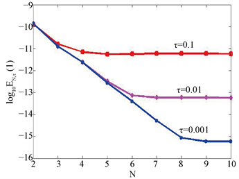
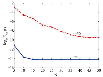
上式中的 $κ$ 和 $x_{0}$ 是任意参数。用如下的无穷范数

$E_{N, τ} (t) = \max_{0 \leq j \leq N} | u (x_{j}, t) - w_{N}^{(β)} (x_{j}, t) |$

计算数值解与理论解之间的误差。图(a)给出 $t = 1$ 时不同时间步长 $τ$ 对应的误差 $E_{N, τ} (t)$ 的常用对数 $\log_{10} E_{N, τ} (t)$ 随N的变化关系。可以发现，数值误差 $E_{N, τ} (1)$ 只须空间节点数 $N \geq 8$ ，时间步长 $τ \leq 0.001$ 时，误差即达到 $O (10^{- 14})$ 量级，说明所提算法格式有谱精度；图(b)与图(a)相比较，就是理论解(12)中的参数 $κ$ 由0.3变为0.5，插值函数中的伸缩因子 $β$ 由1变为1.5。可以看出，算法格式(9)对(10)式中的参数 $κ$ 有较强的适应性，当 $κ$ 较大时插值基函数中的 $β$ 也适当的变大，空间方向仍可以达到谱精度；而已有的文献通常对较小的 $κ$ 逼近精确解(10)，所以算法格式(9)对参数 $κ$ 是稳定的，这是所提算法的一个优点。图(c)给出时间t分别取1和50时的误差变化，当 $t \geq 50$ 时，需要增加节点个数，所提算法格式仍然有效。图(d)是选取插值函数中的伸缩因子 $β$ 不同的值时的误差，表明对孤波解而言，当选择较大的 $β$ 时，数值误差 $E_{N, τ} (1)$ 会变的小一些， $β$ 的值通过试验得到的，理论上还没有解决如何选取最好的 $β$ 值。

(a) $β = 1, κ = 0.3, x_{0} = - 20$ (b) $β = 1.5, κ = 0.5, x_{0} = - 20$

4. 结论

为了避免通常的等距节点Lagrange插值多项式当次数较高时( $N \geq 10$ )出现Runge现象，而采用Gauss型节点构造Lagrange插值多项式逼近问题(1)解。考虑到问题(1)的孤波解的性态，当 $| x | \to + \infty$ 时，其迅速衰减为零，用含有因子 $e^{- β x / 2}$ 的插值函数可以使逼近函数与问题(1)的理论解更好的吻合，从而得到较高精度的数值解。特别，所给算法也适合于(10)中较大的参数 $κ$ 及变量时间t值，表明算法格式(9)是强健的。

基金项目

国家自然科学基金项目(11371123)；SRTP (N.2019198)。

文章引用

王其霞,苗伊浩,王天军. 半直线上Kortewego-de Vries方程的Laguerre谱配置方法
Generalized Laguerre Spectral-Collocation Method for KdV Equations on the Half Line[J]. 应用数学进展, 2020, 09(09): 1583-1588. https://doi.org/10.12677/AAM.2020.99186

参考文献

1. Korteweg, D. and De Vries, G. (1895) On the Change of Form of Long Waves Advancing in a Rectangular Canal, and on a New Type of Long Stationary Waves. Philosophical Magazine, 39, 422-443. https://doi.org/10.1080/14786449508620739

2. Kawahara, R. (1972) Oscillatory Solitary Waves in Dispersive Media. Journal of the Physical Society of Japan, 33, 260-264. https://doi.org/10.1143/JPSJ.33.260

3. Kichenassamy, S. and Olver, P.J. (1992) Existence and Nonexistence of Solitary Wave Solutions to Higher-Order Model Evolution Equations. SIAM Journal on Mathematical Analysis, 23, 1141-1166. https://doi.org/10.1137/0523064

4. 程斌. 用 Petrov-Galerkin 有限元法数值模拟 KdV方程[J]. 数值计算与计算机应用, 1992, 13(1): 73-80.

5. Shen, J. (2003) A New Dual-Petrov-Galerkin Method for Third and Higher Odd-Order Differential Equations: Application to the KdV Equation. SIAM Journal on Numerical Analysis, 41, 1595-1619. https://doi.org/10.1137/S0036142902410271

6. Aksan, E.N. and Zdes, A. (2006) Numerical Solution of Korteweg-De Vries Equation by Galerkin B-Spline Finite Element Method. Applied Mathematics and Computation, 175, 1256-1265. https://doi.org/10.1016/j.amc.2005.08.038

7. 李冰冰, 王天军. Kortewego-Devries 方程的Hermite函数谱配置方法[J]. 应用数学进展, 2019, 8(4): 631-637.

8. 贾红丽, 王中庆. KdV方程的Chebyshev-Hermite谱配置法[J]. 应用数学与计算数学学报, 2013, 27(1): 1-8.

9. 王天军. 半无界非线性热传导方程的Laguerre拟谱方法[J]. 应用数学与计算数学学报, 2013, 27(1): 9-15.

10. Shen, J., Tang, T. and Wang, L.L. (2011) Spectral Mathod: Algorithms, Analysis and Applications. Springer-Verlag, Berlin.

11. Shen, J. and Tang, T. (2006) Spectral and High-Order Methods with Applications. Science Press, Beijing.

期刊菜单