Advances in Applied Mathematics
Vol.
12
No.
07
(
2023
), Article ID:
69657
,
17
pages
10.12677/AAM.2023.127337
非守恒双曲方程组的路径守恒ADER间断Galerkin方法:在浅水方程中的应用
赵晓旭,刘仁迪,钱守国,李刚*
青岛大学数学与统计学院,山东 青岛
收稿日期:2023年6月25日;录用日期:2023年7月19日;发布日期:2023年7月28日

摘要
本文提出了求解非守恒双曲型偏微分方程的一种新的路径守恒间断Galerkin (DG)方法。特别地,这里的方法采用了一级ADER (在空间和时间的任意导数)方法来实现时间离散化。此外,该方法采用微分变换(DT)过程而不是Cauchy-Kowalewski (C-K)过程来实现局部时间演化。与经典的ADER方法相比,该方法不需要求解内部单元的广义黎曼问题。与RKDG (Runge-Kutta DG)方法相比,该方法不需要中间步骤,因此需要较少的计算机存储空间。简而言之,当前的方法是一步一步完全离散的。而且,该方法在空间和时间上都容易获得高阶精度。浅水方程的数值结果表明,该方法具有较高的阶精度,对间断解具有较好的分辨率。
关键词
非守恒双曲方程组,ADER的方法,DG方法,DT过程

A Path-Conservative ADER Discontinuous Galerkin Method for Non-Conservative Hyperbolic Equations: Applications in Shallow Water Equations
Xiaoxu Zhao, Rendi Liu, Shouguo Qian, Gang Li*
School of Mathematics and Statistics, Qingdao University, Qingdao Shandong
Received: Jun. 25th, 2023; accepted: Jul. 19th, 2023; published: Jul. 28th, 2023

ABSTRACT
In this article, we propose a new path-conservative discontinuous Galerkin (DG) method to solve the non-conservative hyperbolic partial differential equations (PDE). In particular, the method here applies the one-stage ADER (Arbitrary DERivatives in space and time) approach to fulfill the temporal discretization. In addition, this method uses the differential transformation (DT) procedure other than the Cauchy-Kowalewski (C-K) procedure to achieve the local temporal evolution. Compared with the classical ADER methods, the current method is free of solving generalized Riemann problems at inter-cells. In comparison with the Runge-Kutta DG (RKDG) methods, the proposed method needs less computer storage thanks to no intermediate stages. In brief, this current method is one-step, one-stage, and fully-discrete. Moreover, this method can easily obtain arbitrary high-order accuracy in space and in time. Numerical results for shallow water equations (SWEs) show that the method enjoys high-order accuracy and keeps good resolutions for discontinuous solutions.
Keywords:Non-Conservative Hyperbolic Equations, ADER Approach, DG Method, DT Procedure

Copyright © 2023 by author(s) and Hans Publishers Inc.
This work is licensed under the Creative Commons Attribution International License (CC BY 4.0).
http://creativecommons.org/licenses/by/4.0/


1. 引言
物理学和工程领域的许多流体问题都可以根据第一原理描述为守恒定律
(1)
其中 为守恒变量向量, 为物理通量张量。到目前为止,我们可以通过守恒原
理深刻地理解自然界中的大多数物理运动。然而,在空气动力学、天体物理学、航空航天、石油工业等领域对可压缩多相流/介质流的建模中,由于不同相(介质)之间复杂的相互作用,出现了非守恒积项(即未知解的空间导数)。因此,相关的数学模型不能以守恒形式表示。然而,上述流体问题可以用拟线性非守恒双曲方程组表示如下
(2)
其中 为方程组矩阵。这里使用分块矩阵语法给出矩阵 和 的紧凑符号。其中,假设方程(2)为双曲型,即 和 分别具有m个实特征值和m个线性无关的特征向量的完整集合。特别地,如果 和 是 和 的雅可比矩阵,则方程(2)将简化为守恒定
律(1)的双曲方程。这一观察结果表明,方程(2)适合同时表示守恒定律和非守恒方程组。
然而,方程(2)的主要问题在于间断情况下弱解的经典定义的不足。直到Dal Maso、Le Floch和Murat的理论(DLM理论) [1] 的出现,这一重大问题才有了很大的进展。DLM理论给出了方程组(2)弱解的定义,通过引入路径 连接相空间中的两个状态 和 。随后,针对DLM理论 [1] ,Castro [2] 和Pares [3] 根据非守恒双曲方程组发展了路径守恒方法(2)。实际上,路径守恒方法 [2] [3] [4] 也可以被称为Toumi [5] 对Roe方法弱表述的扩展。
后来,继最初的成果 [1] [2] 之后,许多研究者对路径守恒方法进行了许多尝试。代表性研究主要有:ADER格式 [6] [7] [8] 、FORCE格式 [9] [10] 、HLLC Riemann解算方法 [11] [12] 、Osher Riemann解算方法 [13] [14] 、中心格式 [15] 、中心迎风格式 [4] [16] 、ADER-DG方法 [17] 等。关于最新进展和简要的历史回顾,我们参考文献 [18] 和 [19] 。
本研究的主要目的是针对非守恒双曲型方程组提出一种新的路径守恒DG方法(2)。该方法采用单阶段ADER方法实现高阶时间离散化,因此称为路径守恒ADER-DG方法。其基本思想是采用DT过程 [20] [21] [22] 代替C-K过程,通过低阶空间展开系数来表示解的时间展开系数。此外,DT过程可以实现任意高阶精度的局部时间演化。就我们而言,这将是第一次尝试将DG方法与DT过程一起应用于非守恒方程组。然后,我们将该方法推广到以非守恒形式处理SWEs。特别是Li等 [17] 提出了一种以双曲平衡律形式求解SWEs的ADER-DG方法。此外,Li [23] 等人将ADER-DG方法推广到求解气体动力学中的欧拉方程。在此,对于非保守形式的SWEs,ADER-DG方法的成功将说明ADER-DG方法具有通用性。
本文的结构如下:第2节阐述了路径守恒的ADER-DG方法的一般框架,然后将所得方法以非守恒形式应用于一维浅水波方程。第3节实现了典型算例来验证所提出方法的性能。第4节给出了一些结论。
2. 路径守恒的ADER-DG法的一般公式
本文针对非守恒方程组(2)给出了一种一般的ADER-DG方法框架。实际上,我们首先将方程组(2)在
给定的近似空间中乘以一个测试函数 ,然后在一个时间单元 上积分,得到
在这里 是空间单元。然后,我们用 作为时间多项式近似。由于 通常在单元间出现跳跃,我们提出了一种路径守恒方法来处理跳跃。
接下来,我们得到PDE(6)的DG方法:对于任意测试函数 ,数值解 满足以下等式
(3)
其中 为单元 边界处的单位向外法向量。
DG方法(3)采用ADER方法实现时间离散化。因此,DG方法(3)是一层一层完全离散的。因此,我
们将提出的方法(3)称为ADER-DG方法。此外,为了实现时间离散,我们需要通过DT过程实现 在时间单元 中的局部时间演化。DT过程将在第2.1.3节中详细描述。这里, 来自单元内部 和 来自单元 外部。此外,符号 表示单元间的跳跃项,满足以下要求 [2] [3] [6] :
· 对于每一个 和 ,
· 对于每一个 , 和 ,
另外, 表示连接状态 和 的足够光滑的路径。满足上述条件的方法称为路
径守恒方法。
此外,根据 [17] [23] ,所提出的求解守恒定律(1)双曲方程组的ADER-DG方法(3)的守恒等价如下
(4)
以 为数值通量近似单元间物理通量 。实际上,当非守恒方程组(2)满足守恒
律(1),即A和B分别是f和g的雅可比矩阵时,上述非守恒形式的路径守恒式ADER-DG方法(3)可简化为保守的ADER-DG方法(4)。Dumbser等人在有限体积格式的框架下对这种等价性进行了详细的证明 [6] 。
2.1. 一维SWEs的应用
基于路径保守的ADER-DG方法的一般框架,我们取以下一维SWEs为例
(5)
来说明该方法(3)的具体实现步骤。式中, 、 分别为水深、流体速度。符号 代表底部地形,字母“g”代表重力加速度。
按照 [2] 中的方法,我们将(5)中的几何源项合并到项 中,得到如下的非守恒形式
(6)
在这里
用 表示声速。这种操作使方程组(6)更易于获得Well-balanced方法。
从数学的观点来看,非守恒方程组(6)保留稳态解,满足
特别地,静止水域的稳态解有以下几种形式
传统的方法不能准确地保持这种稳定状态,并导致非物理振荡。Well-balanced (W-B)方法 [24] [25] 可以在离散水平上保持达到机器精度的稳态,并且即使在相对粗糙的网格上也可以解决稳态的小扰动 [26] ,从而相应地提高计算效率。
2.1.1. 符号和解空间
首先,将空间域 离散成N个空间单元,其中 。这里取 和 作为网格中心和单元 的大小。最大网格尺寸定义为 。这里,我们应用 作为时间单元,并令
(7)
作为近似空间,其中 表示时间单元 上的一组时间多项式,其阶数最高为k。
2.1.2. 一维路径保守的ADER-DG方法的构建
对于以为方程组(6),ADER-DG方法(3)如下:对于 ,解 满足下列等式
(8)
进而,方程(8)也有如下的等式形式
(9)
对于单元间的跳转项 有不同的选择,例如
· Osher跳跃项:
(10)
· Roe跳跃项:
(11)
其中, 为Toumi等在 [5] 中定义的某种意义上 的Roe线性化矩阵,即函数 满足以
下性质:
- 对每个 ,矩阵 具有m个不同的实特征值
- 兼容性属性
- 对于任意 ,矩阵 满足下式要求
根据广义Roe的性质。
另外,对于式(10)和式(11)中矩阵的绝对值算子,我们通常使用以下符号
其中 是矩阵 的右特征向量的矩阵, 表示它的逆矩阵。
目前为止,可以将当前方法(9)视为给定路径 的函数,形式如下
并且,函数 是Lipschitz连续的,满足一定的正则性和相容条件
在本文中,我们应用简单的分段路径
(12)
比如 [2] [3] [6] 。
这种路径的选择十分有用的,它保证了前文所提出的方法对于SWEs [2] [3] [6] 是W-B的。此外,由路径(12),Osher跳跃项(10)可简化为以下形式
(13)
同时,Roe跳跃项(11)可简化为以下形式
(14)
对于式(13)和式(14)中路径积分的计算,我们采用了具有适当高阶精度的高斯正交规则。
2.1.3. DT算法
为了构建方法(9),我们需要提前实现从 开始的时间单元的局部时间演化。这个操作的原因是我们需要在每个时间单元中以多项式的形式得到数值解。然后,我们可以在(9)中以高阶精度计算时间积分和时间积分。实际上,为了实现这一目标,ADER方法 [27] [28] [29] [30] [31] 使用C-K过程反复微分控制PDE,并通过空间导数得到时间导数。为了获得高阶时间精度,我们需要高阶时间导数。此时,由于链式规则的使用,C-K程序将变得非常繁琐。Dumbser和Munz [31] 利用Leibnize规则提出了一种高效的算法。最近,Dumbser等人 [6] [7] ,Tang等人 [32] 应用局部DG预测方法 [29] 来代替C-K程序。最近,Li等人通过DT程序开发了一种针对SWEs的ADER-DG方法 [17] 。
在本研究中,我们采用DT程序而不是C-K程序。实际上,DT过程最初是针对非线性初值问题发展起来的 [33] [34] 。随后,Ayaz将DT过程推广到二维情况 [20] 以及方程组情况 [21] 。Kurnaza等 [22] 将其推广到更一般的n维情况。此外,Norman和Finkel [33] 应用该方法构建了一维SWEs的多矩有限体积格式。
下面我们给出DT过程的具体定义,如 [20] [21] [22] 所示。假设函数 在单元格 是已知的,则DT定义如下
(15)
其中, 表示根据原函数 变换后的函数。
实际上, 表示关于 的展开系数用截断泰勒级数的形式表示。表1显示了这里使用的
一些转换后的函数。

Table 1. Transformed functions of some functions
表1. 部分函数的变换函数
然后,具体说明了DT过程的实现步骤。一开始,我们得到
使用 投影来近似单元格 中的 以及 。
随后,我们对式(5)的两端施加DT过程,得到如下递归式
(16)
在这里,我们使用以下辅助变量
然后,将 , 和 , 带入(16),即可递归得到
结果就是 。
每个空间单元 中的 。此外,为了更好地理解这一过程,我们
给出了DT过程的详细算法。
备注1. 总而言之,DT过程的关键功能是根据现有解 为每个空间单元局部提供高阶时间演化。
备注2. C-K过程直接使用控制PDE的符号展开,并且需要重新计算许多项。因此,C-K过程根据复杂度导致指数增长。然而,DT过程相对简单,但复杂性是可以预测的。
备注3. 在实践中,不需要根据底部地形b应用DT过程,因为底部b只依赖于空间变量x。
2.1.4. 斜率限制器
一般来说,对于间断问题,斜率限制器是必不可少的。在这里,我们使用总变分界(TVB)限制器 [35]
来控制非物理振荡。事实上,我们只根据数值解 来实现TVB限制器步骤,不包括与时间t无关的底部形貌 。具体来说,我们需要在单元平均的基础上识别出“坏单元”(即包含间断的单元)从 在 上的 和单元平均值 。
为了便于说明,我们首先给出一些符号
(17)
然后,我们得到下面更新后的值
对(17)中的变量使用TVB限制器 [35] 。这里, 是一个最小模函数
。单元 被识别为坏单元,只要
随后,单元极限值 被定义为
(18)
最后,根据有限的单元值(18)和单元平均值确定多项式 。
2.1.5. 一维路径守恒的ADER-DG方法的实施步骤
对于以为方程组(6),在一个时间区间 内,本文方法的具体步骤如下:
1) 最初,由 得到
.
2) 使用递归步(16),根据 从 在 处得到 ,并在每个 上得到 。
3) 根据(13)和(14)构造跳跃项 。
4) 用一级公式(9)更新 。
5) 需要时,在 上使用TVB斜率限制器。
6) 重复步骤2)~5)。
3. 数值结果
在此,我们用几个典型的算例来证明所提出的方法。在所有的算例中,我们都在近似空间中使用了二阶以上的时间多项式(即 )。为了保证数值的稳定性,我们取Courant-Friedrichs-Levy (CFL)数值为0.18。另外,我们设重力常数 。为了节省空间,由于Roe类型方法保持了W-B性质,因此我们只使用带有Roe类型跳跃项的方法来呈现数值结果。
3.1. W-B性能测试
首先,我们用一个算例数值证明了W-B性质,如 [36] 。初始条件为
数值证明了Well-balanced性质。特别是,我们在以下两种不同的底部上进行计算:
其中第一个底部是光滑的,而第二个底部是间断的。
表2和表3分别给出了在 时根据两种不同的底部地形产生的误差。很明显,所有的误差都在机器精度的同一量级,故而预期的W-B性能是相应实现的。
Table 2. Errors according to the example over the first bottom
表2. 根据第一个底部的算例得出的误差
Table 3. Errors according to the example over the second bottom
表3. 根据第二个底部的算例得出的误差
3.2. 精度测试
接下来,我们用 [36] 中的一个算例,以及相应的底部地形和初始条件来证明其准确性。初始条件为
在底部上 。
由于解析解无法得到,我们首先需要在一个32,000单元的精细网格上计算这个例子直到t = 0.1 s,然后将得到的数值解作为参考。随后,我们计算t = 0.1 s时的L1误差,并根据参考解得到精度阶数,如表4所示。得到了明显的三阶精度。
Table 4. Errors and accuracy orders for h and hu
表4. h和hu的误差和精度阶
3.3. 稳态水流的扰动
在这里,我们应用 [37] 中的一个算例来测试所提出的方法在凹凸形状底部地形捕捉小扰动的能力。初始数据为
其中 作为凹凸的参数
随着时间的推移,初始扰动分解为两个脉冲,沿两个不同的方向运动,如图1所示,与文献 [37] [38] 中的数值结果保持高度一致。显然,这两种类型的脉冲都可以很好地分解。
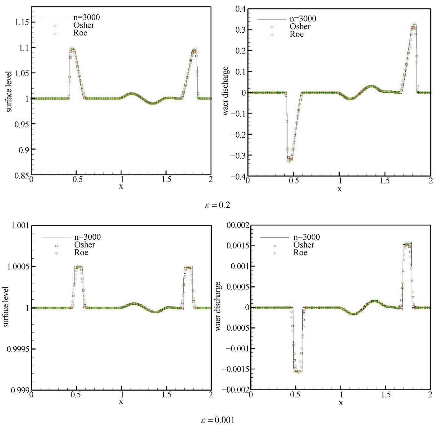
Figure 1. Surface level (left) and water discharge (right) at t = 0.2
图1. t = 0.2时的地表水位(左)和水量(右)
3.4. 矩形底部的溃坝问题
接下来,我们处理一个溃坝问题 [38] [39] [40] ,并使用以下初始条件
在矩形底部上方有
图2分别给出了 和 时的数值解,表明该方法得到了很好的数值解果,与文献 [38] [39] [40] 中的数值解保持一致。

Figure 2. Surface level at t = 15 (left) and t = 60 (right)
图2. t = 15 s (左)和t = 60 s (右)时的表面水平
3.5. 经过驼峰的稳定水流
进而,我们使用一个广泛应用的算例来验证该方法 [41] 。实际上,这个算例是基于初始条件对跨临界和亚临界流进行建模的
越过驼峰
随后,我们在空间区间的两端施加不同的边界条件,计算到t = 200 s。此外,我们还展示了精确解 [42] 加以比较,从而更直观地验证我们的方法。
· 算例A:无激波的跨临界流动
上游边界的流量 ;下游边界的水深 。图3中的Case A的结果表明,数值结果同实际结果相吻合。
· 算例B:带激波的跨临界流动
上游边界的流量 ;下游边界的水深 。图3中的Case B的结果表明,数值结果与精确解有良好的一致性,无伪震荡。
· 算例C:亚临界流
上游边界的流量 ;下游边界的水深 。图3中的Case C的结果表明,数值解和精确解的拟合效果良好。

Figure 3. Surface level h + b at t = 200 s
图3. t = 200 s时的表面水位h + b
3.6. 跨过台阶的溃坝问题
这里,我们利用一个经过台阶的溃坝算例来测试我们的数值方法,以下算例可以很好地测试所构造的方法的鲁棒性。
· 算例A
首先,我们使用以下初始数据实现 [43] 中的算例
跨过一个台阶状底部
随着时间的推移,这个算例产生了向左移动的稀疏波向右移动的激波。
· 算例B
初始条件为
在上面相同的底部。随着时间的推移,这个算例发展出两个朝着不同方向移动的冲击。
· 算例C
本算例来自 [13] ,初始数据为
越过一个台阶
· 算例D
初始数据为
在与算例C相同的底部。
图4为同一网格200个单元在t = 1时的数值结果,与精确的结果吻合较好。我们可以清楚地发现数值结果和精确解保持高度一致,并拥有陡峭的间断过渡。
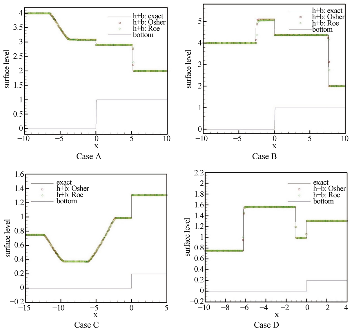
Figure 4. Surface level at t = 1
图4. t = 1时的表面水平
4. 结论
本文针对非保守双曲方程组,提出了一种新的DG方法。该方法采用一阶ADER方法实现时间离散化。然后,我们将该方法应用于求解SWEs。为了实现局部时间的高阶演化,本文采用DT过程代替C-K过程,由空间膨胀系数递归得到时间膨胀系数。与C-K程序相比,DT程序更简洁,编程更方便。此外,由于该方法不需要中间阶段,因此需要较少的计算机存储空间,并且不需要求解单元间的广义黎曼问题。由于该方法具有明确的一步性和紧凑的模板结构,因此它是超级计算机并行计算的理想选择。我们可以很容易地在空间和时间上进行任意高阶精度,而不需要太多的编码工作。基于DT程序。总之,所提出的方法是一步一步完全离散的。此外,大量的数值结果表明,该方法具有高阶精度、良好的平衡性和对间断解的良好分辨率。
基金项目
本研究得到了山东省自然科学基金面上项目(No. ZR2021MA072,ZR2023MA012)的资助。
文章引用
赵晓旭,刘仁迪,钱守国,李 刚. 非守恒双曲方程组的路径守恒ADER间断Galerkin方法:在浅水方程中的应用
A Path-Conservative ADER Discontinuous Galerkin Method for Non-Conservative Hyperbolic Equations: Applications in Shallow Water Equations[J]. 应用数学进展, 2023, 12(07): 3381-3397. https://doi.org/10.12677/AAM.2023.127337
参考文献
- 1. Dal Maso, G., LeFloch, P.G. and Murat, F. (1995) Definition and Weak Stability of Nonconservative Products. Journal de Mathématiques Pures et Appliqués, 74, 483-548.
- 2. Castro, M.J., Gallardo, J.M. and Parés, C.M. (2006) High-Order Finite Volume Schemes Based on Reconstruction of States for Solving Hyperbolic Systems with Noncon-servative Products. Applications to Shallow-Water Systems. Maththematics of Computation, 75, 1103-1134. https://doi.org/10.1090/S0025-5718-06-01851-5
- 3. Parés, C. (2006) Numerical Methods for Nonconservative Hyperbolic Systems: A Theoretical Framework. SIAM Journal on Numerical Analysis, 44, 300-321. https://doi.org/10.1137/050628052
- 4. Diaz, M.J.C., Kurganov, A. and de Luna, T.M. (2019) Path-Conservative Central-Upwind Schemes for Nonconservative Hyperbolic Systems. Mathematical Modelling and Numerical Analysis, 53, 959-985. https://doi.org/10.1051/m2an/2018077
- 5. Toumi, I. (1992) A Weak Formulation of Roes Approximate Riemann Solver. Journal of Computational Physics, 102, 360-373. https://doi.org/10.1016/0021-9991(92)90378-C
- 6. Dumbser, M., Castro, M., Parés, C. and Toro, E.F. (2009) ADER Schemes on Unstructured Meshes for Nonconservative Hyperbolic Systems: Applications to Geophysical Flows. Computers & Fluids, 38, 1731-1748. https://doi.org/10.1016/j.compfluid.2009.03.008
- 7. Dumbser, M., Hidalgo, A. and Zanotti, O. (2014) High Order Space-Time Adaptive ADER-WENO Finite Volume Schemes for Non-Conservative Hyperbolic Systems. Computer Methods in Applied Mechanics and Engineering, 268, 359-387. https://doi.org/10.1016/j.cma.2013.09.022
- 8. Schoeder, S., Kormann, K., Wall, W.A. and Kronbichler, M. (2019) Efficient Explicit Time Stepping of High Order Discontinuous Galerkin Schemes for Waves. SIAM Journal on Scientific Computing, 40, C803-C826. https://doi.org/10.1137/18M1185399
- 9. Dumbser, M., Hidalgo, A., Castro, M.J., Parés, C. and Toro, E.F. (2010) FORCE Schemes on Unstrucktured Meshes II: Nonconservative Hyperbolic Systems. Computer Methods in Applied Mechanics and Engineering, 199, 625-647. https://doi.org/10.1016/j.cma.2009.10.016
- 10. Zhang, L.Q., Yang, S.L., Zeng, Z., Chen, J., Yin, L.M. and Chew, J.W. (2017) Forcing Scheme Analysis for the Axisymmetric Lattice Boltmann Method under Incompressible Limit. Physical Review E, 95, Article ID: 043311. https://doi.org/10.1103/PhysRevE.95.043311
- 11. Tian, B.L., Toro, E.F. and Castro, C.E. (2011) A Path-Conservative Method for a Five-Equation Model of Two-Phase Flow with an HLLC-Type Riemann Solver. Com-puters & Fluids, 46, 122-132. https://doi.org/10.1016/j.compfluid.2011.01.038
- 12. Simon, S. and Mandal, J.C. (2019) A Simple Cure for Nu-merical Shock Instability in the HLLC Riemann Solver. Journal of Computational Physics, 378, 477-496. https://doi.org/10.1016/j.jcp.2018.11.022
- 13. Dumbser, M. and Toro, E.F. (2011) A Simple Extension of the Osher Riemann Solver to Non-Conservative Hyperbolic Systems. Journal of Scientific Computing, 48, 70-88. https://doi.org/10.1007/s10915-010-9400-3
- 14. Dumbser, M. and Toro, E.F. (2011) On Universal Osher-Type Schemes for General Nonlinear Hyperbolic Conservation Laws. Communications in Computational Physics, 10, 635-671. https://doi.org/10.4208/cicp.170610.021210a
- 15. Castro, M.J., Parés, C., Puppo, G. and Russo, G. (2012) Central Schemes for Nonconservative Hyperbolic Systems. SIAM Journal on Scientific Computing, 34, B523-B558. https://doi.org/10.1137/110828873
- 16. Chu, S.S., Kurganov, A. and Na, M.Y. (2022) Fifth-Order A-WENO Schemes Based on the Path-Conservative Central-Upwind Method. Journal of Computational Physics, 469, Article ID: 111508. https://doi.org/10.1016/j.jcp.2022.111508
- 17. Li, G., Li, J.J., Qian, S.G. and Gao, J.M. (2021) A Well-Balanced ADER Discontinuous Galerkin Method Based on Differential Transformation Procedure for Shallow Water Equations. Applied Mathematics and Computation, 395, Article ID: 125848. https://doi.org/10.1016/j.amc.2020.125848
- 18. Parés, C. (2014) Path-Conservative Numerical Methods for Non-conservative Hyperbolic Systems. In: Benzoni-Gavage, S. and Serre, D., Eds., Hyperbolic Problems: Theory, Numerics, Applications, Springer, Berlin, 817-824.
- 19. Castro, M.J., Asunción, M., Fernández-Nieto, E.D., Gallardo, J.M., Gon-ziez Vida, J.M., Macías, J., Moraies, T., Ortega, S. and Parés, C. (2018) A Review on High Order Well-Balanced Path-Conservative Finite Volume Schemes for Geophysical Flows. Proceedings of the International Congress of Math-ematicians, 4, 3533-3558.
- 20. Ayaz, F. (2003) On the Two-Dimensional Differential Transform Method. Applied Mathematics and Computation, 143, 361-374. https://doi.org/10.1016/S0096-3003(02)00368-5
- 21. Ayaz, F. (2004) Solutions of the System of Differential Equations by Differential Transform Method. Applied Mathematics and Computation, 147, 547-567. https://doi.org/10.1016/S0096-3003(02)00794-4
- 22. Kurnaza, A., Oturanc, G. and Kiris, M.E. (2005) n-Dimensional Differential Transformation Method for Solving PDEs. International Journal of Computer Mathematics, 82, 369-380. https://doi.org/10.1080/0020716042000301725
- 23. Zhang, Y.J., Li, G., Qian, S.G. and Gao, J.M. (2021) A New ADER Discontinuous Galerkin Method Based on Differential Transformation Procedure for Hyperbolic Conservation Laws. Computational and Applied Mathematics, 40, Article No. 139. https://doi.org/10.1007/s40314-021-01525-3
- 24. Greenberg, J.M. and Leroux, A.Y. (1996) A Well-Balanced Scheme for the Numerical Processing of Source Terms in Hyperbolic Equations. SIAM Journal on Numerical Analysis, 33, 1-16. https://doi.org/10.1137/0733001
- 25. Greenberg, J.M., Leroux, A.Y., Baraille, R. and Noussair, A. (1997) Analysis and Approximation of Conservation Laws with Source Terms. SIAM Journal on Numerical Analysis, 34, 1980-2007. https://doi.org/10.1137/S0036142995286751
- 26. Noelle, S., Xing, Y.L. and Shu, C.W. (2010) High-Order Well-Balanced Schemes. In: Puppo, G. and Russo, G., Eds., Numerical Methods for Balance Laws, Aachen, 10 August 2010, 25-45.
- 27. Dumbser, M. (2005) Arbitrary High Order Schemes for the Solution of Hyperbolic Conservation Laws in Complex Domains. Shaker Verlag, Aachen.
- 28. Dumbser, M. and Munz, C.D. (2005) Arbitrary High Order Discontinuous Galerkin Schemes. In: Cordier, S., Goudon, T., Gutnic, M. and Sonnendrucker, E. Eds., Numerical Methods for Hyperbolic and Kinetic Problems, EMS Publishing House, 295-333. https://doi.org/10.4171/012-1/13
- 29. Toro, E.F., Millington, R.C. and Nejad, L.A.M. (2001) Towards Very High Order Godunov Schemes. In: Toro, E.F., Ed., Godunov Methods, Springer, New York, 905-938. https://doi.org/10.1007/978-1-4615-0663-8_87
- 30. Titarev, V.A. and Toro, E.F. (2005) ADER Schemes for Three-Dimensional Non-Linear Hyperbolic Systems. Journal of Computational Physics, 204, 715-736. https://doi.org/10.1016/j.jcp.2004.10.028
- 31. Dumbser, M. and Munz, C.D. (2006) Building Blocks for Arbitrary High Order Discontinuous Galerkin Schemes. Journal of Scientific Computing, 27, 215-230. https://doi.org/10.1007/s10915-005-9025-0
- 32. Duan, J. and Tang, H. (2020) An Efficient ADER Discontinuous Galerkin Scheme for Directly Solving Hamilton-Jacobi Equation. Journal of Computational Mathematics, 38, 58-83. https://doi.org/10.4208/jcm.1902-m2018-0189
- 33. Pukhov, G.E. (1982) Differential Transforms and Circuit The-ory. International Journal of Circuit Theory and Applications, 10, 265-276. https://doi.org/10.1002/cta.4490100307
- 34. Zhou, J.K. (1986) Differential Transformation and Its Applications for Electrical Circuits. Huazhong University Press, Wuhan.
- 35. Shu, C.W. (1988) Total-Variation-Diminishing Time Dis-cretizations. SIAM Journal on Scientific and Statistical Computting, 9, 1073-1084. https://doi.org/10.1137/0909073
- 36. Xing, Y.L. and Shu, C.W. (2005) High Order Finite Difference WENO Schemes with the Exact Conservation Property for the Shallow Water Equations. Journal of Computational Physics, 208, 206-227. https://doi.org/10.1016/j.jcp.2005.02.006
- 37. LeVeque, R.J. (1998) Balancing Source Terms and Flux Gradient on High-Resolution Godunov Methods: The Quasi-Steady Wave-Propagation Algorithm. Journal of Computational Physics, 146, 346-365. https://doi.org/10.1006/jcph.1998.6058
- 38. Xing, Y.L. and Shu, C.W. (2006) A New Approach of High Order Well-Balanced Finite Volume WENO Schemes and Discontinuous Galerkin Methods for a Class of Hyperbolic Systems with Source Terms. Communications in Computational Physics, 1, 100-134.
- 39. Vukovic, S. and Sopta, L. (2002) ENO and WENO Schemes with the Exact Conservation Property for One-Dimensional Shallow Water Equations. Jour-nal of Computational Physics, 179, 593-621. https://doi.org/10.1006/jcph.2002.7076
- 40. Li, G., Caleff, V. and Qi, Z.K. (2015) A Well-Balanced Finite Differ-ence WENO Scheme for Shallow Water Flow Model. Applied Mathematics and Computation, 265, 1-16. https://doi.org/10.1016/j.amc.2015.04.054
- 41. Vazquez-Cendon, M.E. (1999) Improved Treatment of Source Terms in Upwind Schemes for the Shallow Water Equations in Channels with Irregular Geometry. Journal of Computa-tional Physics, 148, 497-526. https://doi.org/10.1006/jcph.1998.6127
- 42. Annunziato, A., Dogan, G. and Yalciner, A. (2023) Modeling Dam Break Events Using Shallow Water Model. Eng, 4, 1851-1870. https://doi.org/10.3390/eng4030105
- 43. Alcrudo, F. and Benkhaldoun, F. (2001) Exact Solutions to the Rie-mann Problem of the Shallow Water Equations with a Bottom Step. Computers & Fluids, 30, 643-671. https://doi.org/10.1016/S0045-7930(01)00013-5
NOTES
*通讯作者。