Operations Research and Fuzziology
Vol.08 No.02(2018), Article ID:25164,8
pages
10.12677/ORF.2018.82007
Synchronization and Local Convergence Analysis of Complex Dynamical Networks with Nodes Delay
Jingwen Mu, Caixia Gao
School of Mathematical Science, Inner Mongolia University, Hohhot Inner Mongolia

Received: May 9th, 2018; accepted: May 21st, 2018; published: May 29th, 2018

ABSTRACT
In recent years, synchronization of complex networks has received an increasing attention due to their wide applications in many fields. To analyze and reveal the inherent mechanism of local synchronization in the complex networks with delayed nodes, this paper attempts to investigate it by the Lyapunov direct method which can be utilized as a theoretical methodology. First, we investigated local synchronization of complex networks with delayed nodes by this method and obtained some sufficient conditions to guarantee the networks reaching local synchronization. The criterion is very simple and can be readily applied in the real world networks. Then, an example is provided to verify the effectiveness of the main results.
Keywords:Synchronization, Local Convergence, Complex Networks, Delayed Nodes, Lyapunov Direct Method
具有节点时滞的复杂网络的同步 和局部收敛性分析
慕静文,高彩霞
内蒙古大学数学科学学院,内蒙古 呼和浩特
收稿日期:2018年5月9日;录用日期:2018年5月21日;发布日期:2018年5月29日

摘 要
近年来,由于复杂网络的同步在许多领域有着广泛的应用,因此受到了越来越多的关注。为了分析和揭示具有时滞节点的复杂网络的局部同步的内在机制,本文采用Lyapunov直接法进行理论分析研究。首先,我们采用这种方法研究了具有时滞节点的复杂网络的局部同步,给出了保证网络实现局部同步的充分条件。该判据条件简单,便于在实际网络中应用。然后,通过一个算例验证了主要结果的有效性。
关键词 :同步,局部收敛性,复杂网络,时滞节点,Lyapunov直接法

Copyright © 2018 by authors and Hans Publishers Inc.
This work is licensed under the Creative Commons Attribution International License (CC BY).
http://creativecommons.org/licenses/by/4.0/


1. 引言
一个复杂网络是由一组互相连接的节点组成的,每个节点在不同的研究体系下的意义是不同的。现在,复杂网络的研究已经成为科学界的一个热点,引起了很多领域的科学家的关注。随着Internet的发展,复杂网络已经走进了我们的生活,许多自然和人工系统都可以用网络来表达,如神经网络 [1] 、计算机网络 [2] 、万维网 [3] 、社会网络 [4] 等。
时滞在现实生活中十分常见,因而在复杂网络系统中,时滞的影响是不可避免的 [5] [6] 。如病毒的传播,病毒会占用时间,传播的广度和深度会影响网络的拓扑结构和耦合结构。虽然系统引入时滞会变得更复杂,但考虑时滞是十分必要的。近十几年来,许多学者对具有时滞的复杂网络进行了大量的研究,得到了很多优秀的成果。李等 [7] 在已有的复杂网络的模型中引入耦合时滞,对含有耦合时滞的复杂网络的稳定定性进行了研究;徐等 [8] 进一步的对含有耦合时滞的复杂网络进行了研究,并且给出了同步准则。张等 [9] 研究了节点含有时滞的复杂网络稳定性问题。孙等 [10] 在非线性耦合系统中引入节点时滞,考虑了节点时滞对网络稳定性的影响,对其进行了稳定性研究。
人们首先注意到同步是观察两个时钟的同步运动:两个时钟不管从初始位置是什么,一段时间后它们会同步摆动。同步现在被认为是一种集体活动,研究发现许多现实世界中的问题在网络中有着密切的关系 [11] [12] 。例如,因特网同步,哺乳动物大脑中神经元的同步 [13] 。研究网络同步有许多优点,对于一些有害的同步效应,如网络同步,周期性路由信息同步,我们希望这些同步消除。现在,这种非常普遍而又重要的现象引起了许多科学家的关注。萧帆望和关蓉晨 [14] [15] 研究了耦合振荡器的网络同步问题,是一个连续系统的稳定性问题。吴等 [16] 研究了随机有向网络的同步问题。李等 [17] 研究了一类具有时变时滞的复杂网络的局部和全局同步问题。
本文的主要内容安排如下。第1节给出问题的描述及本文用到的预备知识;第2节采用Lyapunov直接法给出了复杂网络实现局部同步的充分条件,并且进行证明;第3节通过一个算例来验证所得结论的有效性;第4节为本文的小结。
2. 预备知识
考虑一个由m个相同时滞节点组成的复杂动态网络,每个节点都是一个n维非自治动力系统。其描如下:
(1)
其中 是第i个节点的状态, , 表示常时滞, 为网络节点间的耦合矩阵, 表示节点j对节点i的耦合权重 , 表示内连耦合矩阵, 是一个连续可微函数。
首先给出本文所需的一些定义、假设和引理。
假设:对于时滞微分方程 ,其中 , 是一个连续函数,则对于任意初始条件 都存在一个唯一的连续解。
定义1: [18] 令 是网络(1)的一个解,其中 。假设 和 是连续的。若存在一个非空子集 和 ,使得对所有的 都有 ,并且
其中 ,则称复杂网络(1)实现了渐进同步, 称为复杂网络同步的同步区域。
定义2: [19] 矩阵 称为属于 类的,若
1) 。
2) A的特征值均具有负实部,除了单特征值0。
定义3: [19] 矩阵 称为属于 类的,若
1) ;
2) A是不可约的。
引理1: [20] 若 ,则有
1) 若λ是A的特征值, ,则 。
2) A必有一个单特征值 ,且其对应的右特征向量为 。
3) 假设 (不失一般性,假设 )是A对应于特征值0的左特征向量,则对所有的 ,均有 。
4) 若 ,则对所有的 ,当且仅当 成立。
5) 若A是可约的,当且仅当存在某些下标i,有 。此时,经过适当的置换变换,可假设 ,其中 满足 ,且
满足 , 。则A可分解成 ,其中 是不可约的,且 。
3. 主要结果
对于复杂网络(1),假设 ,则有:
(2)
邻接矩阵A对应的Laplacian矩阵 定义为 ,则(2)可以化为:
(3)
引入记号 ,其中 为矩阵L的0特征值对应的左特征向量,满足 。由于 ,则 的动态方程可以描述为
(4)
定义误差向量 ,利用线性化方法,可得 满足的变分方程:
其中 是函数 在 处的雅克比矩阵。 是函数 在 处的雅克比阵。
记 ,则(5)的矩阵形式为
(5)
令矩阵L的Jordan分解为 ,其中 是对角阵, 是矩阵L的特征值。令 ,则 的变分方程为
(6)
定理1:由于S第一列是A对应特征值0的特征向量,由前面分析可知,因此只需考虑 , 个变分方程。若 ,则变分方程
(7)
是渐进稳定的,则复杂网络(1)是局部同步稳定的。
定理2:设L的特征值全为实数, 来记雅克比矩阵 , 来记雅克比矩阵 对于 ,都存在正常数 ,其中 ,使得
(8)
成立,则复杂网络(1)是局部稳定的。
证明:设 ,由条件(8)可知,存在 ,当 时,有
(9)
对于任意的 ,定义Lyapunov泛函
(10)
对 求导得
对充分大的t都成立。进一步,对 成立,必然对 都成立。因此,复杂网络(1)对 都是稳定的,由定理1,可知本定理得证。
4. 算例
在本小节,给出一个具体的算例来验证上一节的主要结论。
考虑一个由50个节点组成的复杂网络,每个节点的时滞 ,每个节点的动力学方程可以描述为
(11)
其中 。
假设内部耦合矩阵 ,网络是完全联通的。网络的Laplacian矩阵为
矩阵L的特征值为 。
图1~图3描述了复杂网络第i个节点的三个分量 的同步误差 ,由图

Figure 1. Synchronization error for the first component xi1 of the i-th node
图1. 第i个节点的第1个分量xi1的同步误差

Figure 2. Synchronization error for the second component xi2 of the i-th node
图2. 第i个节点的第2个分量xi2的同步误差
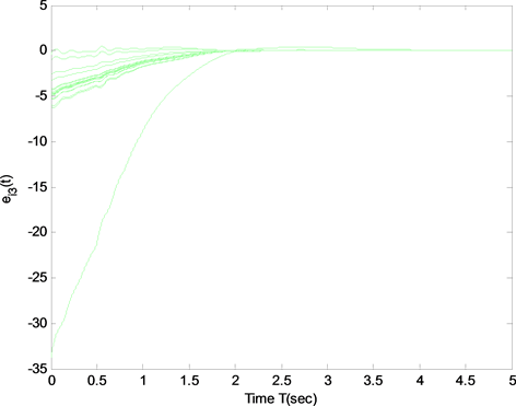
Figure 3. Synchronization error for the third component xi3 of the i-th node
图3. 第i个节点的第3个分量xi3的同步误差
可知所有的同步误差均能快速的收敛到0,从而可以得到复杂网络(11)最终会随时间趋于同步。
5. 结论
本文研究了具有节点时滞的复杂网络的局部同步。首先,采用Lyapunov直接法给出了保证复杂网络局部同步的充分条件;其次,通过一个具体的算例说明了这种方法的有效性。具有节点时滞的复杂网络的同步问题的研究仍然具有很大的挑战性,下一步,我们将对具有节点时滞的时变网络的局部同步问题进行研究。
文章引用
慕静文,高彩霞. 具有节点时滞的复杂网络的同步和局部收敛性分析
Synchronization and Local Convergence Analysis of Complex Dynamical Networks with Nodes Delay[J]. 运筹与模糊学, 2018, 08(02): 54-61. https://doi.org/10.12677/ORF.2018.82007
参考文献
- 1. Döfler, F. and Bullo, F. (2014) Synchronization in Complex Networks of Phase Oscillators: A Survey. Automatica, 56, 1539-1564. https://doi.org/10.1016/j.automatica.2014.04.012
- 2. Pastor-Satorras, R. and Vespignani, A. (2004) Evolution and Structure of the Internet. Cambridge University Press, Cambridge. https://doi.org/10.1017/CBO9780511610905
- 3. Huberman, B.A. and Adamic, LA. (1999) Internet: Growth Dynamics of the World Wide Web. Nature, 401, 131. https://doi.org/10.1038/43604
- 4. Baych, C.T. and Galvani, A.P. (2013) Social Factors in Epidemiology. Science, 342, 47-49. https://doi.org/10.1126/science.1244492
- 5. Pyragas, K. (1998) Synchronization of Coupled Time-Delay Systems: Analytical Estimations. Physical Review E, 58, 3067-3071. https://doi.org/10.1103/PhysRevE.58.3067
- 6. Mensour, B. and Longtin, A. (2004) Synchronization in Coupled Map Lattices with Small-World Delayed Interactions. Physica A, 35, 365-370.
- 7. Li, C. and Chen, G. (2004) Synchronization in General Complex Dynamical Networks with Coupling Delays. Physica A, 343, 236-278. https://doi.org/10.1016/j.physa.2004.05.058
- 8. Xu, S.Y. and Yang, Y. (2009) Synchronization for a Class of Complex Dynamical Networks with Time-Delay. Communications in Nonlinear Science and Numerical Simulation, 14, 3230-3238. https://doi.org/10.1016/j.cnsns.2008.12.022
- 9. Zhang, Q., Lu, J. and Lv, J. (2008) Adaptive Feedback Syn-chronization of a General Complex Dynamical Network with Delayed Nodes. IEEE Transitions on Circuits and Systems II: Express Briefs, 55, 183-187. https://doi.org/10.1109/TCSII.2007.911813
- 10. Sun, W., Chen, Z. and Kang, Y.H. (2012) Impulsive Synchronization of a Nonlinear Coupled Complex Network with a Delay Node. Chinese Physics B, 21, Article ID: 010504. https://doi.org/10.1088/1674-1056/21/1/010504
- 11. Strogate, S.H. (2001) Exploring Complex Network. Nature, 410, 268-276. https://doi.org/10.1038/35065725
- 12. Albert, R. and Barabási, A.L. (2002) Statistical Mechanics of Complex Networks. Reviews of Modern Physics, 74, 47-97. https://doi.org/10.1103/RevModPhys.74.47
- 13. Bennett, M.L. and Zukin, R.S. (2004) Electrical Coupling and Neuronal Synchronization in the Mammalian Brain. Neuron, 41, 495-511. https://doi.org/10.1016/S0896-6273(04)00043-1
- 14. Wang, X.F. and Chen, G. (2002) Synchronization in Scale-Free Dynamical Networks: Robustness and Fragility. IEEE Trans Circuits System I, 49, 54-62. https://doi.org/10.1109/81.974874
- 15. Wang, X.F. and Chen, G. (2002) Synchronization in Small-World Dynamical Networks. International Journal of Bifurcation and Chaos, 12, 187-182. https://doi.org/10.1142/S0218127402004292
- 16. Wu, C.W. (2006) Synchronization and Convergence of Linear Dynamics in Random Directed Networks. IEEE Transactions on Automatic Control, 51, 1207-1210. https://doi.org/10.1109/TAC.2006.878783
- 17. Li, P., Zhang, Y. and Zhang, L. (2006) Global Synchronization of a Class of Delayed Complex Networks. Chaos, Solitons & Fractals, 30, 903-908. https://doi.org/10.1016/j.chaos.2005.08.169
- 18. Lü, J., Yu, X. and Chen, G. (2004) Chaos Synchronization of General Complex Dynamical Networks. Journal of Physics A, 334, 281-302. https://doi.org/10.1016/j.physa.2003.10.052
- 19. 路君安, 刘慧, 陈娟. 复杂动态网络的同步[M]. 北京: 高等教育出版社, 2016.
- 20. Horn, P.A. and Johnson, C.R. (1985) Matrix Analysis. Cambridge University Press, New York. https://doi.org/10.1017/CBO9780511810817