Advances in Applied Mathematics
Vol.07 No.08(2018), Article ID:26534,13
pages
10.12677/AAM.2018.78116
Dynamic Analysis of a Predator-Prey System with Time Delay and Pulse Control
Jing Yang
College of Mathematics Physics and Electronic Information Engineering, Wenzhou University, Wenzhou Zhejiang

Received: Aug. 1st, 2018; accepted: Aug. 15th, 2018; published: Aug. 22nd, 2018

ABSTRACT
Based on theory of ecological dynamics and ecological control modeling idea, a predator-prey dynamic system with time-delay and pulse control is constructed. The sufficient criterion of local asymptotic stability and global attraction for the semi-trivial periodic solution of the system is established. The permanence of the system is proved. Further, the dynamic behavior of the model was simulated numerically, which verifies the validity and feasibility of theoretical analysis.
Keywords:Pulse Control, Time Delay, Stability, Global Attraction, Persistence
一类具有时滞效应与脉冲控制的捕食–食饵系统的动力学研究
杨晶
温州大学,数理与电子信息工程学院,浙江 温州
收稿日期:2018年8月1日;录用日期:2018年8月15日;发布日期:2018年8月22日

摘 要
基于生态动力学理论与生态控制建模思想,本文构建了一类具有时滞效应与脉冲控制的捕食–食饵动力系统,建立了系统半平凡周期解的局部渐近稳定和全局吸引的充分判据,证明了系统的持久生存性。对模型相关动力学行为进行数值模拟,验证了理论分析的有效性和可行性。
关键词 :脉冲控制,时滞效应,稳定性,全局吸引,持久性

Copyright © 2018 by author and Hans Publishers Inc.
This work is licensed under the Creative Commons Attribution International License (CC BY).
http://creativecommons.org/licenses/by/4.0/


1. 引言
随着社会的发展和科学技术的进步,许多先进控制技术都被应用于抑制害虫的研究中,但是害虫仍然还在持续的增长。关于害虫的治理一般有两种方法 [1] :一种是化学控制 [2] ,即通过喷洒杀虫剂来控制害虫的数量,最终消灭害虫;另一种是生物防治 [3] [4] [5] ,即利用其它生物来消灭或抑制害虫。如论文 [6] 主要研究了一类控制害虫的动力学模型,即通过捕食者释放、栖息地管理和杀虫剂释放来确定控制的可行性以及对种群均衡的影响。研究结果表明在无天敌情况下,生境管理或农药释放的控制将有效地对抗被攻击阶段;在有捕食者存在的条件下,使用栖息地管理或释放杀虫剂的效果在很大程度上取决于捕食者是否在高密度下相互干扰。
捕食与被捕食关系是种群生态学中最重要的相互制约关系,捕食–食饵动力学系统是生物数学研究的重要研究对象。关于捕获问题的理论讨论已有较长的历史,在Lotka和Volterra [7] 做出开创性工作之后,这个理论的讨论直到今天也是值得学者们关注的。捕食–食饵动力系统的建模基础方程主要有常微分方程(ODEs) [8] 、时滞微分方程 [9] 、偏微分方程(PDEs) [10] 等。近几年,具有脉冲控制策略的微分方程模型已引起了越来越多人的注意,已构建了一些具有脉冲控制的捕食–食饵模型 [11] - [18] ,它们可以解决很多实际的生物学问题。如论文 [19] 从解析和数值上研究了具有异地养分输入、脉冲扰动控制和季节扰动的生态模型,得到了维持某些物种灭绝和所有物种持久性的充分判据,数值工作显示影响长期动态行为的关键因素是脉冲扰动和异地养分输入,并发现季节性干扰的外来养分输入能够加剧周期性震荡,促进混沌出现。
年龄结构是种群建模中最重要的特征之一,将个体分为幼年和成年两类是最简单的年龄结构。在种群完整的生命阶段,种群的幼年和成年个体有着完全不同的食物链关系、不同的生存空间和不同的疏散特征,这些特征在昆虫和两栖动物中尤其明显,它们通常拥有幼年阶段并经历蜕变的过程 [20] 。通常幼年捕食者或者食饵从出生到成熟需要一定的时间;即使幼年捕食者或者食饵的死亡率非零,也仅有一部分捕食者或者食饵可以存活到成年。因此在现实的捕食–食饵模型中考虑种群的年龄结构 [21] [22] [23] [24] [25] ,同时讨论年龄结构对捕食–食饵种群动力学性态的影响具有一定现实意义。如Chen等人在1992年提出了一类具有年龄结构的单种群生态模型,若令 , 分别代表幼虫和成虫在t时刻的密度,则在 [26] 建立了一类具有年龄结构的单种群生态模型,表示如下:
(1)
其中, 代表幼虫在t时刻的出生率, , 分别是幼虫和成虫在t时刻的死亡率, 代表幼虫转化为成虫的转化率, 代表成功从幼虫转化为成虫的比例系数。Aiello,Freedman [27] 对上面的模型(1)继续研究,引入年龄结构,得到
(2)
其中, 分别代表幼虫和成虫在t时刻的密度, 是幼虫转化为成虫的时间常数, 是正常数。本论文在系统(2)的基础上,考虑了不同时刻害虫防治的周期性扰动控制和化学控制,研究了一类三种群捕食–食饵动力系统。利用Floquet定理等理论获得了一个渐近稳定的半平凡周期解,当捕食者的释放量大于临界值时,杀虫效果比较好。
基于以上讨论和分析,设 表示食饵的密度;r表示内增长率;a表示常数,则有
(3)
随着营养物质的吸收,食饵会从幼虫变为成虫,此时令 表示幼虫状态下的食饵, 表示成虫状态下的食饵,则有 。如果食饵的天敌 出现,则捕食者会捕食食饵。若假设在食饵量多及状态明显的情况下,捕食者仅捕食处于成虫状态下的食饵,且捕食的功能反应项为 ,则有
(4)
其中, 代表在 时刻幼虫食饵出生并且在t时刻一直存活, 代表幼虫食饵转化为成虫食饵的时间段, 分别代表幼虫食饵,成虫食饵与食饵天敌的死亡率,k代表能源转化率。
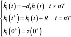
对上述模型引入周期脉冲,则有
(5)
其中, , , , ,R表示在 时刻,人工投入的捕食者的量,T代表脉冲周期, , 。
同时,假设系统(5)的初值条件满足:
(6)
除此之外,考虑到系统(5)的生物学意义,假设
(7)
2. 定理
下面引入一些关于数学的概念,定义和引理等。
若令 , , 是系统(5)中前三个方程的右导数,令 ,则 。
如果1)对任意的 ,在区间 内,V是连续的且有 存在;
2) V对于X满足局部的Lipschitz条件。
定义2.1假设 是系统(5)的任意解,在满足初值条件 下,一定存在常数 ,使得对任意的 都有 成立,则系统(5)是持久的。
引理2.1 (见 [28] )假设 满足
(8)
其中, 且 是常数,则对任意的 ,有
关于这个定理的证明过程,可以查阅 [28] 。当系统(8)所有的不定式的方向都相反时,相似的结论也可以得到。
引理2.2 (见 [28] )考虑下面的脉冲微分方程:
(9)
则系统(9)有唯一的正周期解 ,且对系统(9)的任意解 都有 成立,其中,
.
引理2.3 (见 [29] )考虑时滞微分方程:
, (10)
其中 ,对任意的 有 ,且 在 内是连续的, ,则有
1) 若 ,则 ;
2) 若 ,则 。
引理2.4 (见 [29] )考虑时滞微分方程:
, (11)
其中对任意的 有 ,则有
1) 若 ,则 ;
2) 若 ,则 。
3. 理论分析
3.1. 系统(5)任意解的有界性
定理3.1设 是系统(5)的任意解,则一定存在常数 ,使得对任意的 有 。
证明:定义函数 , 。
当 时,
因为 是有界的, , 是有界的,则有
又当 时, 。
考虑系统
(12)
依据引理2.1和引理2.2,系统(12)的解
(13)
所以知 是有界的,
即证。
3.2. 系统(5)半平凡周期解的局部渐近稳定性
定理3.2如果满足条件 , ,则系统(5)的半平凡周期解 是局部渐近稳定的,其中 , , , 。
证明:系统(5)的半平凡周期解 可以通过引理2.2直接求知。设 ,对系统(5)作线性化处理,得到
(14)
若设当 时, 为基础矩阵,且满足
(15)
其中,
当 时, 。
所以系统(14)的单值矩阵 。
又依据系统(15),知
(16)
其中, 。
若假设 为 的特征根,则
(17)
根据脉冲微分方程的Floquet定理 [30] ,若 ,则系统(5)的半平凡周期解 是局部渐近稳定的。
另,令 是系统(15)的任意解,则
. (18)
所以知 。
3.3. 系统(5)半平凡周期解的全局吸引性
定理3.3如果 ,则系统(5)的半平凡周期解 是全局吸引的。
证明:由系统(5)的第三个方程,有
 (19)
(19)
考虑方程组:
 (20)
(20)
依据引理2.2,知 ,且
,且
 . (21)
所以一定存在 ,使得
,使得 。
。
所以由系统(5)的第二个方程知
 (22)
(22)
考虑微分方程
 (23)
(23)
依据引理2.4,若 ,则
,则 。
。
又由引理2.1,系统(22)的解 。
。
所以根据 和比较原则,知
 。
。
即对任意的 ,存在
,存在 使得对一切的
 都有
都有 。
。
再根据系统(5)的第三个方程,有
 (24)
(24)
依据引理2.1,系统(24)的解
其中, 是系统(25)的解。
 (25)
(25)
且 是系统(26)的解。
 (26)
(26)
且有 。
。
 。
。
所以对任意的 ,存在
,存在 ,使得
,使得 。
。
又因为当 时,
时, 。
。
所以 。
。
即 。
。
由系统(5)的第一个方程,有 ,对上述方程在
 积分有
积分有
 (27)
(27)
其中,

因为定理3.2满足

所以当 时,有
时,有 。
。
所以当 时,有
时,有 。
。
即 。
。
即证。
3.4. 系统(5)的持久生存性
定理3.4如果 ,则系统(5)的任意解
 ,一定存在
,一定存在 ,使得
,使得 ,
, ,
, ,即系统(5)是持久生存性的。
证明:由定理3.1,一定存在 ,使得对于系统(5)的任意解
 ,满足
,满足 ,
, 。
。
由 ,知对任意的
 ,存在
,存在 ,使得
,使得 。
。
即一定存在 ,使得
,使得 。
。
所以只需证明存在 ,使得对任意的
 ,都有
,都有 即可。
即可。
对于系统(5)的第二个方程,有
 (28)
(28)
若设 ,则
,则
 (29)
(29)
若条件 成立,则对
成立,则对 ,会使得
,会使得 ,其中
,其中 。
。
(H1):假设对上面的 ,对任意的
,对任意的 ,当
,当 时,有
时,有 不恒成立,则可以假设存在
 ,使得当
,使得当 时有
时有 成立。
成立。
根据系统(5)的第三个方程,有
 (30)
(30)
考虑系统:
 (31)
(31)
求解系统有
 (32)
(32)
根据引理2.1有
 (33)
(33)
又根据定理3.1,系统(29)有
 (34)
(34)
若设 ,则对任意的
 ,有
,有 。否则,存在一个
 ,使得当
,使得当 时,有
时,有 且
且 ,
, 。
。
又根据系统(5)的第二个方程,
 (35)
(35)
这与 矛盾。所以对任意的
 都有
都有 成立,从而对任意的
 都有
都有 成立。所以知当
 时,
时, ,这与
,这与 矛盾,所以第一个假设成立。
(H2):根据第一个假设,只需要考虑两种情况,
1)对所有的充分大的t,都有 成立;
成立;
2)当t充分大时, 关于
关于 左右波动。
左右波动。
对于情况1),显然成立;因此只需考虑情况2)。
定义 ,其中
,其中
 (36)
(36)
下证明对于充分大的t,有 。由已知,存在
 ,
, ,使得对所有的
 ,有
,有 ,其中当
,其中当 充分大时,有
 成立。又根据定理3.1有界性,知
 是一致连续的。所以系统(5)的正解是一致有界的且不受脉冲影响。因此,存在一个
 ,使得对任意的
 都有
都有 成立。若
成立。若 ,则显然;若
 ,则根据系统(5)的第二个方程,可以得到
 。则知当
。则知当 时,有
时,有 成立。重复上面(H1)的过程,可得
 ,
, 结论。
结论。
又因为区间 (
( 充分大)的任意性,所以当t充分大时,仍有
 成立。即2)得证。
又对于系统(5)的第一个方程,有
 (37)
(37)
由比较定理有 。
。
所以取 ,
, ,
,
则根据定义2.1即证。
4. 数值模拟
若假设 ,
, ,
, ,
, ,
, ,
, ,
, ,
, ,
, ,
, 且初值
且初值 ,
, ,
, 。则根据图1,可以看到当
 时,系统(5)的半平凡周期解
 是局部渐近稳定的,从而验证了定理3.2的有效性。
若假设 ,
, ,
, ,
, ,
, ,
, ,
, ,
, ,
, 且初值
且初值 ,
, ,
, 。根据图2可知:当
 时,系统(5)是持久生存的,从而验证了定理3.4的有效性。
5. 结论
本论文构建了一类具有时滞效应和脉冲控制的捕食–食饵动力系统,对其相关动力学性质进行研究。首先,探讨了系统(5)的半平凡周期解的局部渐近稳定性与全局吸引性,获得了相关的充分判据。其次,探索了系统(5)的种群持久生存性,给出了维持种群持久生存的阈值条件。最后,借助数值模拟工作验证了理论推导工作的有效性。
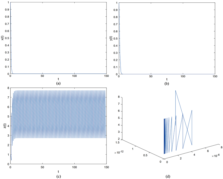
Figure 1. Time diagram and phase diagram of system (5) when 
图1. 当 时,系统(5)的时序图与相位图
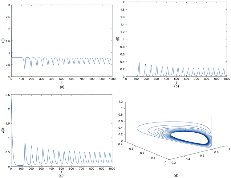
Figure 2. Time diagram and phase diagram of system (5) when 
图2. 当 时,系统(5)时序图与相位图
基金项目
国家自然科学基金面上项目(31570364)。
文章引用
杨晶. 一类具有时滞效应与脉冲控制的捕食–食饵系统的动力学研究
Dynamic Analysis of a Predator-Prey System with Time Delay and Pulse Control[J]. 应用数学进展, 2018, 07(08): 987-999. https://doi.org/10.12677/AAM.2018.78116
参考文献
- 1. 宋燕, 杜月, 李紫薇. 具有阶段结构及脉冲控制的害虫管理模型[J]. 渤海大学学报(自然科学版), 2017, 38(2): 104-110.
- 2. Cai, S., Jiao, J. and Li, L. (2015) Dynamics of a Pest Management Predator-Prey Model with Stage Structure and Im-pulsive Stocking. Journal of Applied Mathematics & Computing, 52, 125-138. https://doi.org/10.1007/s12190-015-0933-3
- 3. Grasman, J., van Herwaarden, O.A., Hemerik, L. and van Lenteren, J.C. (2001) A Two-Component Model of Host-Parasitoid Interactions: Determination of the Size of Inundative Releases of Parasitoids in Biological Pest Control. Mathematical Biosciences, 169, 207-216. https://doi.org/10.1016/S0025-5564(00)00051-1
- 4. Liu, X. and Chen, L. (2003) Complex Dynamics of Holling Type ii Lotka-Volterra Predator-Prey System with Impulsive Perturbations on the Predator. Chaos Solitons & Fractals, 16, 311-320. https://doi.org/10.1016/S0960-0779(02)00408-3
- 5. Panetta, J.C. (1996) A Mathematical Model of Periodically Pulsed Che-motherapy: Tumor Recurrence and Metastasis in a Competitive Environment. Bulletin of Mathematical Biology, 58, 425-447. https://doi.org/10.1007/BF02460591
- 6. Barclay, H.J. (1982) Models for Pest Control Using Predator Release, Habitat Man-agement and Pesticide Release in Combination. Journal of Applied Ecology, 19, 337-348. https://doi.org/10.2307/2403471
- 7. Lotka, A.J. (1927) Scientific Books: Elements of Physical Biology. Science, 66, 281-282. https://doi.org/10.1126/science.66.1708.281-a
- 8. Hethcote, H.W., Wang, W., Han, L. and Ma, Z. (2004) A Predator-Prey Model with Infected Prey. Theoretical Population Biology, 66, 259-268. https://doi.org/10.1016/j.tpb.2004.06.010
- 9. Liu, S. and Beretta, E. (2006) A Stage-Structured Predator-Prey Model of Beddington-Deangelis Type. Siam Journal on Applied Mathematics, 66, 1101-1129. https://doi.org/10.1137/050630003
- 10. Gourley, S.A. and Lou, Y. (2014) A Mathematical Model for the Spatial Spread and Biocontrol of the Asian Longhorned Beetle. Siam Journal on Applied Mathematics, 74, 2-11. https://doi.org/10.1137/130939304
- 11. Yu, H., Zhao, M., Wang, Q. and Agarwal, R.P. (2014) A Focus on Long-Run Sustai-nability of an Impulsive Switched Eutrophication Controlling System Based upon the Zeya Reservoir. Journal of the Franklin Institute, 351, 487-499. https://doi.org/10.1016/j.jfranklin.2013.08.025
- 12. Zhang, Y., Chen, S., Gao, S. and Wei, X. (2017) Stochastic Periodic Solution for a Perturbed Non-Autonomous Predator-Prey Model with Generalized Nonlinear Harvesting and Impulses. Physica A: Statistical Mechanics & Its Applications, 486, 347-366. https://doi.org/10.1016/j.physa.2017.05.058
- 13. Yu, H., Zhong, S. and Agarwal, R.P. (2011) Mathematics Analysis and Chaos in an Ecological Model with an Impulsive Control Strategy. Communications in Nonlinear Science & Numerical Simulation, 16, 776-786. https://doi.org/10.1016/j.cnsns.2010.04.017
- 14. Xie, Y., Wang, L., Deng, Q. and Wu, Z. (2017) The Dynamics of an Impulsive Predator-Prey Model with Communicable Disease in the Prey Species Only. Applied Mathematics & Computation, 292, 320-335. https://doi.org/10.1016/j.amc.2016.07.042
- 15. Wang, Z., Shao, Y., Fang, X. and Ma, X. (2016) The Dynamic Behaviors of One-Predator Two-Prey System with Mutual Interference and Impulsive Control. Mathematics & Computers in Simulation, 132, 68-85. https://doi.org/10.1016/j.matcom.2016.06.007
- 16. Ding, X. and Jiang, J. (2009) Periodicity in a Generalized Semi-Ratio-Dependent Predator-Prey System with Time Delays and Impulses. Journal of Mathematical Analysis & Applications, 360, 223-234. https://doi.org/10.1016/j.jmaa.2009.06.048
- 17. Pei, Y., Liu, S., Li, C. and Chen, L. (2009) The Dynamics of an Impulsive Delay Si Model with Variable Coefficients. Applied Mathematical Modelling, 33, 2766-2776. https://doi.org/10.1016/j.apm.2008.08.011
- 18. Tan, R., Liu, Z. and Cheke, R.A. (2012) Periodicity and Stability in a Sin-gle-Species Model Governed by Impulsive Differential Equation. Applied Mathematical Modelling, 36, 1085-1094. https://doi.org/10.1016/j.apm.2011.07.056
- 19. Dai, C., Zhao, M. and Chen, L. (2012) Complex Dynamic Behavior of Three-Species Ecological Model with Impulse Perturbations and Seasonal Disturbances. Mathematics & Computers in Simulation, 84, 83-97. https://doi.org/10.1016/j.matcom.2012.09.004
- 20. 卢肠. 几类捕食-食饵模型的定性分析[J]. 哈尔滨: 哈尔滨工业大学, 2017.
- 21. Khajanchi, S. and Banerjee, S. (2017) Role of Constant Prey Refuge on Stage Structure Predator-Prey Model with Ratio Dependent Functional Response. Applied Mathematics & Computation, 314, 193-198. https://doi.org/10.1016/j.amc.2017.07.017
- 22. Jiao, J. and Chen, L. (2008) Global Attractivity of a Stage-Structure Variable Coefficients Predator-Prey System with Time Delay and Impulsive Perturbations on Predators. International Journal of Biomathe-matics, 1, 197-208. https://doi.org/10.1142/S1793524508000163
- 23. Zhang, H. and Chen, L. (2008) A Model for Two Species with Stage Structure and Feedback Control. International Journal of Biomathematics, 1, 267-286. https://doi.org/10.1142/S1793524508000230
- 24. Shao, Y. and Ma, X. (2017) Analysis of a Predator-Prey System with Bed-dington-Type Functional Response and Stage-Structure of Prey. International Journal of Dynamical Systems & Differential Equations, 7, 51. https://doi.org/10.1504/IJDSDE.2017.083727
- 25. Sailer, R.I. (1975) Book Review: Biological Control by Natural Ene-mies.
- 26. Chen, F., Xie, X. and Li, Z. (2012) Partial Survival and Extinction of a Delayed Predator-Prey Model with Stage Structure. Applied Mathematics & Computation, 219, 4157-4162. https://doi.org/10.1016/j.amc.2012.10.055
- 27. Aiello, W.G. and Freedman, H.I. (1990) A Time-Delay Model of Single-Species Growth with Stage Structure. Mathematical Biosciences, 101, 139. https://doi.org/10.1016/0025-5564(90)90019-U
- 28. Pei, Y., Li, C. and Fan, S. (2013) A Mathematical Model of a Three Species Prey-Predator System with Impulsive Control and Holling Functional Response. Applied Mathematics and Computation, 219, 10945-10955. https://doi.org/10.1016/j.amc.2013.05.012
- 29. Pang, G., Wang, F. and Chen, L. (2009) Extinction and Permanence in Delayed Stage-Structure Predator-Prey System with Impulsive Effects. Chaos Solitons & Fractals, 39, 2216-2224. https://doi.org/10.1016/j.chaos.2007.06.071
- 30. Bainov, D.D. and Simeonov, P.S. (1995) Impulsive Differential Equations: Asymptotic Properties of the Solutions. World Scientific, Singapore. https://doi.org/10.1142/2413