Dynamical Systems and Control
Vol.07 No.03(2018), Article ID:25757,13
pages
10.12677/DSC.2018.73019
Passivity and Filtering of 2-D Switched Continuous Discrete Systems
Jingbo Gao, Juan Yao*, Weiqun Wang
Nanjing University of Science and Technology, Nanjing Jiangsu

Received: Jun. 4th, 2018; accepted: Jun. 28th, 2018; published: Jul. 5th, 2018

ABSTRACT
The passivity of 2-D switched continuous-discrete systems is discussed. By designing a state dependent switching law that only relies on time, the passivity sufficient conditions are obtained. When there is an external disturbance in 2-D switched continuous-discrete system, passive filters based on observer and general form are designed to ensure the passivity of closed-loop 2-D switched continuous-discrete systems with exogenous disturbance. Two numerical simulations are carried out to verify the validity of the results.
Keywords:2-D Continuous-Discrete Systems, Switching Law, Passivity, Filtering
2-D切换连续离散系统的无源性和滤波
高靖波,姚娟*,王为群
南京理工大学,江苏 南京
收稿日期:2018年6月4日;录用日期:2018年6月28日;发布日期:2018年7月5日

摘 要
本文研究了2-D切换连续离散系统的无源性。通过设计与时间有关的状态依赖切换律,给出了系统无源的充分条件。当2-D切换离散系存在外部扰动时,分别设计了基于观测器和一般形式的无源滤波器,使得闭环2-D 切换连续离散系统是无源的。最后给出了两个数值仿真,来验证所得结论的有效性。
关键词 :2-D切换连续离散系统,切换律,无源性,滤波

Copyright © 2018 by authors and Hans Publishers Inc.
This work is licensed under the Creative Commons Attribution International License (CC BY).
http://creativecommons.org/licenses/by/4.0/


1. 引言
2-D连续离散系统作为一类特殊的2-D系统,它的信息传播在一个方向上连续,在另一个方向上是离散的。2-D连续离散系统与许多实际工程领域紧密相连,如线性重复过程 [1] [2] [3] 、空间互联系统 [4] 、车辆排 [5] 和水渠灌溉 [6] 。关于2-D连续离散系统的渐近稳定性分析和综合已有很多研究。Owens [7] 研究了一类具有动态边界条件的2-D连续线性离散系统的稳定性。Buslowicz [8] 和Kaczorek [9] 分别研究了以Roesser模型和一般模型给出的2-D连续线性离散系统的稳定性。Chesi [10] 给出了混合2-D连续离散系统的稳定性充要条件和性能分析。Wang [11] 基于KYP引理得到了2-D连续离散系统的稳定性和鲁棒稳定性。
另一方面,切换系统是具有有限个连续时间或离散时间子系统和控制这些子系统之间切换的切换规则组成的混杂系统。关于1-D切换系统的研究已有了很多成果 [12] [13] [14] 。在2-D切换系统中,切换律的引入也会影响系统的稳定性,如子系统的稳定性不等同于整个系统的稳定性。目前切换系统中切换律的设计方法有任意切换方法 [15] ,驻留时间方法 [16] [17] 和状态依赖切换方法 [18] 。通过任意切换方法,Benzaouia [19] 首次基于多李雅普诺夫函数考虑了2-D切换系统的稳定性和镇定性问题 [20] 。Shao [21] 讨论了一类具有时滞的线性随机切换系统的鲁棒H∞重复控制问题。平均驻留时间方法也在一些论文中得到应用。Shao [22] 研究了离散时间2-D切换系统的指数稳定和镇定问题。Xiang [23] 给出了二维离散切换系统的输出反馈H∞镇定性分析。Duan [24] 讨论了具有状态时滞的不确定2-D离散切换系统的鲁棒可靠控制器的设计。Shao [25] 对一类切换重复系统设计了迭代学习控制律。通过状态依赖方法,Ghous [26] 研究了2-D切换连续系统的状态反馈H∞控制问题。Bochniak [27] 分析具有奇偶子系统的线性离散重复过程的镇定问题。到目前为止,关于2-D切换系统的研究集中在2-D切换连续系统和2-D连续切换系统上,而没有关于2-D切换连续离散系统的研究。这促使我们开展这方面的研究工作。
耗散性在被Willems [28] 首先提出来后,广泛应用到物理学、应用数学以及力学等领域。耗散性和无源性理论使学者们基于能量输入输出描述给出了控制系统分析和设计的新框架,对系统控制的诸多方面都起到了很大的推动作用。耗散性和无源性理论不仅在控制理论方面有着重要的作用,在许多实际系统,如机器人系统,机电系统,电力系统,内燃机工程,化工过程等的研究中也扮演着很重要的角色。目前对于系统耗散性和无源性的研究大部分集中在1-D系统 [29] [30] [31] [32] 。关于2-D系统的耗散性研究也获得了一些成果 [33] [34] [35] 。可以看到,目前关于2-D系统无源性研究还没有涉及切换情形,特别是对2-D切换离散系统和2-D切换连续离散系统的无源性,无源滤波和反馈无源性是值得研究的问题。
滤波问题是控制系统和信号处理中的一个基本问题,滤波是从含有干扰的接收信号中提取有用信号的一种技术。自从鲁棒滤波方法被引入到系统的状态估计中出现了大量的研究成果。Du [36] 考虑了2-D离散系统的H∞滤波器设计,通过建立2-D离散系统的界实引理,采用Riccati方程方法解决了2-D离散系统的有限范围和无限范围H∞滤波问题。Tuan [37] 基于新的线性矩阵不等式刻画研究了2-D离散系统鲁棒混合H2/H∞滤波问题。还有一些关于2-D系统鲁棒性的研究可见参考文献 [38] [39] [40] 。可以看到,目前关于2-D系统鲁棒性的研究主要集中在2-D离散系统上,关于2-D连续离散系统鲁棒性的研究并不多。
值得注意的是,现有的2-D切换系统 [22] - [27] 的切换规则设计方法都是在斜割直线i + j = l上,这种方法将2-D切换系统看作了一族1-D系统,因此很难推广到2-D切换连续离散系统上,因为对于2-D切换连续离散系统,系统状态x(t, k)中t是时间变量,k是空间变量,t + k是没有意义的。在以上的分析基础上,设计了一个只与时间t有关的状态依赖切换律来研究2-D切换连续离散系统的无源性。
本文组织如下。第二节是问题陈述。第三节对2-D切换连续离散系统,给出系统无源的充分条件。第四节分别设计了基于观测器和一般形式的滤波器,讨论了2-D切换连续离散系统的无源性滤波问题。最后给出了两个数值算例来验证所得结果的有效性。
2. 问题陈述
考虑如下的2-D切换连续离散Roesser模型:
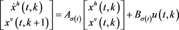 (1)
(1)
(2)
边界条件为: , 。其中 和 分别是水平和垂直状态, 是输出向量。 是切换信号,其中N是子系统个数。 表示第l个子系统是激活的。系数矩阵 是适维常数矩阵,记 。
首先给出2-D切换连续离散系统Roesser模型(1)如下形式的储能函数
(3)
则储能函数沿系统轨迹的散度算子为
(4)
其中 。
借助于储能函数可以定义系统的无源性。
定义1 [41] :2-D连续离散系统(1)称为是无源的,如果存在储能函数使得如下条件成立
(5)
在本章中,我们的目的是给出2-D切换连续离散系统(1)~(2)的无源性条件,然后设计基于观测器和一般形式的滤波器来解决2-D切换连续离散系统(1)~(2)的无源滤波问题。
3. 2-D切换连续离散系统的无源性分析
针对2-D切换连续离散系统(1)~(2),我们给出如下系统无源的充分条件。
定理1:给定常数 ,如果存在正定矩阵 , , 和元素是 的Metzler矩阵 ,使得不等式
(6)
在如下切换律
(7)
成立,其中 ,那么2-D切换连续离散系统(1)是无源的。
证明:选择如下的Lyapunov函数
当 ,即第l个子系统是激活的, 沿系统的任意轨迹的微分满足
的差分满足
于是
由切换律(7)可得
由条件(6)得到
则

由无源性定义1,2-D切换连续离散系统(1)~(2)是无源的。
4. 2-D切换连续离散系统的无源滤波
在本节中,我们将分别设计基于观测器和一般形式的滤波器。考虑如下的带扰动的2-D切换连续离散系统:
(8)
(9)
(10)
边界条件为: , 。其中 和 分别是水平和垂直状态, 是测量输出, 是外部扰动, 是待估信号。 是切换信号,其中N是子系统个数。 表示第l个子系统是激活的。系数矩阵 , , , 是适维常数矩阵。
4.1. 基于观测器的无源滤波器
为2-D切换连续离散系统(8)~(10)设计如下基于观测器的2-D滤波器:
(11)
(12)
其中 , 和 分别是 , 和 的估计,
是滤波器增益。定义滤波误差
, ,
,我们得到如下2-D滤波误差系统:
,
,我们得到如下2-D滤波误差系统:
(13)
(14)
下面我们给出2-D滤波器(11)~(12)是无源滤波器的定义。
定义2 [41] :2-D滤波器(11)~(12)称为是系统(13)~(14)的无源滤波器如果存在储能函数(3)使得如下条件成立
(15)
如下定理给出了2-D切换连续离散系统(8)~(10)存在基于观测器的2-D无源滤波器的充分条件,并且给出了滤波器增益。
定理3.2:给定常数 ,如果存在对称正定矩阵 , ,和矩阵 , , 与元素是 的Metzler矩阵 ,不等式
(16)
在如下切换律
(17)
下成立,其中 ,那么滤波器(11),(12)是2-D切换连续离散系统(8)~(10)的无源滤波器。其中滤波器增益为 , 。
证明:将滤波器增益 , 代入条件(16),再利用Schur补可得条件(6),则对滤波器误差系统(13)~(14)利用定理1可得系统是无源的。
4.2. 一般形式的无源滤波器
本节为2-D切换连续离散系统(8)~(10)设计如下的一般形式2-D滤波器:
(18)
(19)
其中 , , , 是滤波器增益。则2-D 切换连续离散系统(8)-(10)的扩维系统为:
(20)
(21)
其中 , , , , , , , , , , , , 。
下面的定理,给出了2-D切换连续离散系统(8)~(10)在一般形式滤波器(18),(19)下是无源的充分条件,并且给出了滤波器系数矩阵的设计方法。
定理3.3:给定常数 ,如果存在对称正定矩阵 , , 和矩阵 , , , , 与元素是 的Metzler矩阵 ,不等式
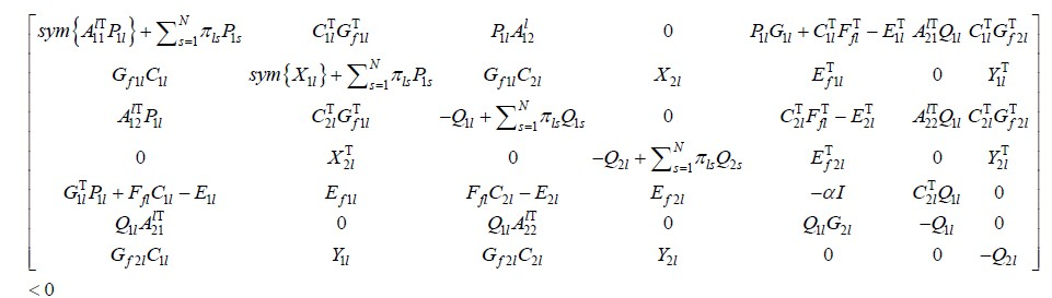 (22)
(22)
在如下切换律
(23)
下成立,其中 ,那么滤波器(18),(19)是2-D切换连续离散系统(8)-(10)的无源滤波器。其中 , 。滤波器增益 。
证明:计算可得 , , 。
对定理1中条件(6)用Schur补可得
(24)
根据如下的对应关系
, ,
, 得到
将滤波器增益 代入(25)即可得2-D切换连续离散系统(8)~(10)是无源的。
5. 数值算例
在本节中,我们给出两个例子说明两类滤波器设计方法的可行性。首先考虑基于观测器的滤波器。
例1:考虑具有两个子系统的2-D切换系统(8)~(10)。
子系统1: ,
,
,
。
,
,
,
。
子系统2: , , , 。
边界条件 , ,令 。根据定理2,可得滤波器增益 , 。则由定理2,切换系统(8)是无源的。2-D滤波误差系统(13)的状态如图1和图2所示,图3给出了系统的切换律。
其次考虑一般形式的滤波器。

Figure 1. State of the 2-D filter error system (13) eh
图1. 2-D滤波误差系统(13)的状态eh
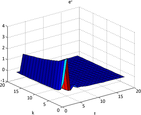
Figure 2. State of the 2-D filter error system (13) ev
图2. 2-D滤波误差系统(13)的状态ev
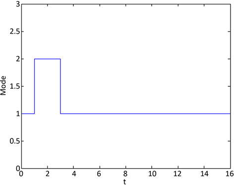
Figure 3. Switching law of the 2-D filter error system (13)
图3. 2-D滤波误差系统(13)的切换律
例2:对具有两个子系统的2-D切换连续离散系统(8)~(10)。
子系统1: , , , 。
子系统2: , , ,
边界条件 , ,令 。根据定理3,可得滤波器增益
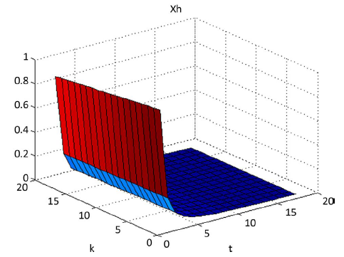
Figure 4. State of the 2-D switched continuous-discrete system (8) xh
图4. 2-D切换连续离散系统(8)的状态xh
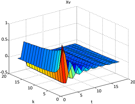
Figure 5. State of the 2-D switched continuous-discrete system (8) xv
图5. 2-D切换连续离散系统(8)的状态xv
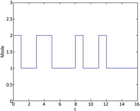
Figure 6. Switching law of 2-D switched continuous-discrete system (8)
图6. 切换律
, , , , , 。则由定理3,2-D切换连续离散系统(8)是无源的。则2-D切换连续离散系统(8)的状态如图4和图5所示,图6给出了系统的切换律。
6. 本文总结
本文研究了2-D切换连续离散系统的无源性和滤波问题。首先通过设计状态依赖切换律得到了2-D切换连续离散系统的无源性充分条件。然后,设计了基于观测器和一般形式的无源滤波器来保证2-D切换连续离散系统在有外部扰动时的无源性,得到了无源滤波器的设计方法。最后,给出两个数值算例验证所得结果的有效性。
基金项目
本文得到“国家自然科学基金青年基金”资助,基金号61603188,在此表示感谢。
文章引用
高靖波,姚 娟,王为群. 2-D切换连续离散系统的无源性和滤波
Passivity and Filtering of 2-D Switched Continuous Discrete Systems[J]. 动力系统与控制, 2018, 07(03): 169-181. https://doi.org/10.12677/DSC.2018.73019
参考文献
- 1. Rogers, E., Galkowski, K. and Owens, D.H. (2007) Control Systems Theory and Applications for Linear Repetitive Processes (Vol. 349). Springer Science & Business Media.
- 2. Bristow, D.A., Tharayil, M. and Alleyne, A.G. (2006) A Survey of Iterative Learning Control. IEEE Control Systems, 26, 96-114.
https://doi.org/10.1109/MCS.2006.1636313 - 3. Hladowski, L., Galkowski, K., Cai, Z., Rogers, E., Freeman, C.T. and Lewin, P.L. (2012) Output Information Based Iterative Learning Control Law Design with Experimental Verification. Journal of Dynamic Systems, Measurement, and Control, 134, 021012.
https://doi.org/10.1115/1.4005038 - 4. D’Andrea, R. and Dullerud, G.E. (2015) Distributed Control Design for Spatially Interconnected Systems. IEEE Transactions on Automatic Control, 48, 1478-1495.
https://doi.org/10.1109/TAC.2003.816954 - 5. Knorn, S. (2013) A Two-Dimensional Systems Stability Analysis of Vehicle Platoons. Doctoral Dissertation, National University of Ireland, Maynooth.
- 6. Li, Y., Cantoni, M. and Weyer, E. (2006) On Water-Level Error Propagation in Controlled Irrigation Channels. Proceedings of the 44th IEEE Conference on Decision and Control, Seville, 15 December 2005, 2101-2106.
- 7. Owens, D.H. and Rogers, E. (1999) Stability Analysis for a Class of 2D Continuous-Discrete Linear Systems with Dynamic Boundary Conditions. Systems & Control Letters, 37, 55-60.
https://doi.org/10.1016/S0167-6911(99)00008-0 - 8. Buslowicz, M. and Ruszewski, A. (2012) Computer Methods for Stability Analysis of the Roesser Type Model of 2D Continuous-Discrete Linear Systems. International Journal of Applied Mathematics and Computer Science, 22, 401-408.
https://doi.org/10.2478/v10006-012-0030-9 - 9. Kaczorek, T. (2011) Stability of Continuous-Discrete Linear Systems Described by the General Model. Technical Sciences, 59, 189-193.
- 10. Chesi, G. and Middleton, R.H. (2014) Necessary and Sufficient LMI Conditions for Stability and Performance Analysis of 2-D Mixed Continu-ous-Discrete-Time Systems. IEEE Transactions on Automatic Control, 59, 996-1007.
https://doi.org/10.1109/TAC.2014.2299353 - 11. Wang, L., Wang, W., Gao, J. and Chen, W. (2017) Stability and Robust Stabilization of 2-D Continuous-Discrete Systems in Roesser Model Based on KYP Lemma. Multidimensional Systems and Signal Processing, 28, 251-264.
https://doi.org/10.1007/s11045-015-0355-2 - 12. Lin, H. and Antsaklis, P. J. (2009) Stability and Stabilizability of Switched Linear Systems: A Survey of Recent Results. IEEE Transactions on Automatic Control, 54, 308-322.
https://doi.org/10.1109/TAC.2008.2012009 - 13. Cheng, J., Xiong, L., Wang, B. and Yang, J. (2015) Robust Fi-nite-Time Boundedness of H∞ Filtering for Switched Systems with Time-Varying Delay. Optimal Control Applications and Methods, 37, No. 2.
- 14. Yin, Y., Zhao, X. and Zheng, X. (2017) New Stability and Stabilization Conditions of Switched Systems with Mode-Dependent Average Dwell Time. Circuits, Systems, and Signal Processing, 36, 82-98.
https://doi.org/10.1007/s00034-016-0306-7 - 15. Balluchi, A., Benedetto, M.D., Pinello, C., Rossi, C. and San-giovanni-Vincentelli, A. (1997) Cut-Off in Engine Control: A Hybrid System Approach. Proceedings of the 36th IEEE Conference on Decision and Control, San Diego, 12 December 1997, 4720-4725.
https://doi.org/10.1109/CDC.1997.649753 - 16. Lian, J., Zhao, J. and Dimirovski, G.M. (2010) Integral Sliding Mode Control for a Class of Uncertain Switched Nonlinear Systems. European Journal of Control, 16, 16-22.
https://doi.org/10.3166/ejc.16.16-22 - 17. Lian, J., Feng, Z. and Shi, P. (2011) Observer Design for Switched Recurrent Neural Networks: An Average Dwell Time Approach. IEEE Transaction on Neural Networks, 22, 1547-1556.
https://doi.org/10.1109/TNN.2011.2162111 - 18. Geromel, J.C. and Colaneri, P. (2006) Stability and Stabilization of Continuous-Time Switched Linear Systems. SIAM Journal on Control and Optimization, 45, 1915-1930.
https://doi.org/10.1137/050646366 - 19. Benzaouia, A., Hmamed, A. and Tadeo, F. (2009) Stability Conditions for Discrete 2D Switching Systems, Based on a Multiple Lyapunov Function. European Control Conference (ECC), Budapest, 23-26 August 2009, 2706-2710.
- 20. Benzaouia, A., Hmamed, A., Tadeo, F. and Hajjaji, A.E. (2011) Stabilisation of Discrete 2D Time Switching Systems by State Feedback Control. International Journal of Systems Science, 42, 479-487.
https://doi.org/10.1080/00207720903576522 - 21. Shao, Z., Huang, S. and Xiang, Z. (2015) Robust H∞ Repetitive Control for a Class of Linear Stochastic Switched Systems with Time Delay. Circuits, Systems, and Signal Processing, 34, 1363-1377.
https://doi.org/10.1007/s00034-014-9905-3 - 22. Xiang, Z. and Huang, S. (2013) Stability Analysis and Stabili-zation of Discrete-Time 2D Switched Systems. Circuits, Systems, and Signal Processing, 32, 401-414.
https://doi.org/10.1007/s00034-012-9464-4 - 23. Duan, Z. and Xiang, Z. (2014) Output Feedback H∞ Stabilization of 2D Discrete Switched Systems in FM LSS Model. Circuits, Systems, and Signal Processing, 33, 1095-1117.
https://doi.org/10.1007/s00034-013-9680-6 - 24. Emelianova, J., Emelianov, M., Pakshin, P., et al. (2015) Dissi-pativity of Nonlinear 2D Systems. IFAC-PapersOnLine, 48, 784-789.
https://doi.org/10.1016/j.ifacol.2015.09.285 - 25. Shao, Z. and Xiang, Z. (2016) Design of an Iterative Learning Control Law for a Class of Switched Repetitive Systems. Circuits, Systems, and Signal Processing, 36, 845-866.
- 26. Ghous, I. and Xiang, Z. (2016) H∞ Control of a Class of 2-D Continuous Switched Delayed Systems via State-Dependent Switching. International Journal of Systems Science, 47, 300-313.
https://doi.org/10.1080/00207721.2015.1068882 - 27. Bochniak, J., Galkowski, K., Rogers, E., Mehdi, D., Bachelier, O. and Kummert, A. (2006) Stabilization of Discrete Linear Repetitive Processes with Switched Dynamics. Multidimensional Systems and Signal Processing, 17, 271-295.
https://doi.org/10.1007/s11045-005-6298-2 - 28. Willems, J.C. (1972) Dissipative Dynamical Systems Part I: General Theory. Archive for Rational Mechanics & Analysis, 45, 321-351.
https://doi.org/10.1007/BF00276493 - 29. Xie, S., Xie, L. and Carlos, E. (1997) Robust Dissipative Control for Linear Systems with Dissipative Uncertainty. Systems & Control Letters, 29, 255-268.
https://doi.org/10.1016/S0167-6911(97)90009-8 - 30. Tan, Z., Soh, Y.C. and Xie, L. (1999) Dissipative Control for Linear Discrete-Time Systems. Automatica, 35, 1557-1564.
https://doi.org/10.1016/S0005-1098(99)00069-2 - 31. Li, Z., Wang, J. and Shao, H. (2002) Delay-Dependent Dissipative Control for Linear Time-Delay Systems. Journal of the Franklin Institute, 339, 529-542.
https://doi.org/10.1016/S0016-0032(02)00030-3 - 32. Wu, Z., Cui, M., Xie, X. and Shi, P. (2011) Theory of Stochastic Dissipative Systems. IEEE Transactions on Automatic Control, 56, 1650-1655.
https://doi.org/10.1109/TAC.2011.2121370 - 33. Ahn, C.K., Shi, P. and Basin, M.V. (2015) Two-Dimensional Dissipative Control and Filtering for Roesser Model. IEEE Transactions on Automatic Control, 60, 1745-1759.
https://doi.org/10.1109/TAC.2015.2398887 - 34. Ahn, C.K. and Kar, H. (2015) Passivity and Finite-Gain Per-formance for Two-Dimensional Digital Filters: The FM LSS Model Case. IEEE Transactions on Circuits and Systems II: Express Briefs, 62, 871-875.
https://doi.org/10.1109/TCSII.2015.2435261 - 35. Wang, L., Chen, W. and Li, L. (2017) Dissipative Stability Analysis and Control of Two-Dimensional Fornasini-Marchesini Local State-Space Model. International Journal of Systems Science, 48, 1744-1751.
https://doi.org/10.1080/00207721.2017.1282059 - 36. Du, C., Xie, L. and Soh, Y. (2000) H∞ Filtering of 2-D Discrete Systems. IEEE Transactions on Signal Processing, 48, 1760-1768.
https://doi.org/10.1109/78.845933 - 37. Tuan, H.D., Apkarian, P., Nguyen, T.Q. and Narikiyo, T. (2002) Robust Mixed H2/H∞ Filtering of 2-D Systems. IEEE Transactions on Signal Processing, 50, 1759-1771.
https://doi.org/10.1109/TSP.2002.1011215 - 38. Hoang, N., Tuan, D., Nguyen, T. and Hosoe, S. (2005) Robust Mixed Generalized H2/H∞ Filtering of 2-D Nonlinear Fractional Transformation Systems. IEEE Transactions on Signal Processing, 53, 4697-4706.
https://doi.org/10.1109/TSP.2005.859259 - 39. Xu, S., Lam, J., Zou, Y., Lin, Z. and Paszke, W. (2005) Robust H∞ Filtering for Uncertain 2-D Continuous Systems. IEEE Transactions on Signal Processing, 53, 1731-1738.
https://doi.org/10.1109/TSP.2005.845464 - 40. Carlos, E., Souza, D., Xie, L. and Daniel, F.C. (2009) Robust Fil-tering for 2-D Discrete-Time Linear Systems with Convex-Bounded Parameter Uncertainty. Automatica, 42, 354-359.
- 41. Pakshin, P., Emelianova, J., Emelianov, M., Gallkowski, K. and Rogers, E. (2016) Dissipativity and Stabilization of Nonlinear Repetitive Processes. Systems & Control Letters, 91, 14-20.
https://doi.org/10.1016/j.sysconle.2016.01.005
NOTES
*通讯作者。