Advances in Applied Mathematics
Vol.
12
No.
10
(
2023
), Article ID:
74494
,
9
pages
10.12677/AAM.2023.1210444
求解具有等式约束的随机优化问题的二阶微分方程方法
吕琪楠,孙菊贺,王莉,谢红俭
沈阳航空航天大学理学院,辽宁 沈阳
收稿日期:2023年9月26日;录用日期:2023年10月21日;发布日期:2023年10月30日

摘要
针对具有等式约束的随机优化问题,本文首先考虑基于SAA方法获取原始问题目标函数的SAA问题,并利用惩罚函数法将其转化为一般无约束凸优化问题。接下来建立二阶微分方程算法对所得到的问题进行求解。本文还证明了当算法的参数满足一定条件时,二阶微分方程算法具有良好的收敛性,其收敛率为 ,最后给出具体的数值算例验证算法的可行性。
关键词
随机优化问题,二阶微分方程算法,凸优化问题,SAA方法

Second Order Differential Equation Algorithm for Solving Stochastic Optimization Problems with Equality Constraints
Qinan Lv, Juhe Sun, Li Wang, Hongjian Xie
School of Science, Shenyang University of Aeronautics and Astronautics, Shenyang Liaoning
Received: Sep. 26th, 2023; accepted: Oct. 21st, 2023; published: Oct. 30th, 2023

ABSTRACT
For the stochastic optimization problem with equality constraint, this paper first considers the SAA problem of obtaining the objective function of the original problem based on the SAA method, and uses the penalty function method to transform it into a general unconstrained convex optimization problem. Next, a second-order differential equation algorithm is established to solve the obtained problem. This paper also proves that when the parameters of the algorithm meet certain conditions, the second-order differential equation algorithm has good convergence, and its convergence rate is , and finally a specific numerical example is given to verify the feasibility of the algorithm.
Keywords:Stochastic Optimization Problem, Second-Order Differential Equation System, Convex Optimization Problem, SAA Method

Copyright © 2023 by author(s) and Hans Publishers Inc.
This work is licensed under the Creative Commons Attribution International License (CC BY 4.0).
http://creativecommons.org/licenses/by/4.0/


1. 引言
随着经济发展,许多实际问题往往存在许多不确定性因素,例如物理不确定性,经济不确定性,统计不确定性等 [1] [2] 。因此,许多学者在研究优化问题时引入了随机变量,得到随机优化问题。随机优化问题作为确定性优化问题的延伸,在机械、经济、人工智能等领域都有很多应用。
随机优化问题首先被G. Dantzig提出,在文献 [3] 中,他提出了带补偿的两阶段随机优化问题,随着经济学和人类需求的进步,越来越多的学者开始关注随机优化问题。同时,针对各种形式的随机优化问题,许多学者给出了不同的算法 [2] [3] [4] [5] [6] 。
针对 形式的问题,Guo等人在文献 [7] 中提出了随机无梯度的Frank-wolf方法,主要解释了目标函数中的随机函数可以证明算法在海德尔连续性条件下的收敛性,无需满足利普希茨的连续性。此外,Guo等人还指出,在算法的收敛分析中,梯度方差是均匀有界的假设是没有必要的。
Curtis等在文献 [8] 中提出了一种基于梯度下降算法方法的随机平均梯度(SAG)计算方法,并证明了一定条件下的线性收敛性。Schmidt等在文献 [9] 中提出了一种基于一阶SGD方法的后续方法。Chen等人在文献 [10] 中将不精确的牛顿方法与随机分解方法相结合,提出了一种解决两阶段随机问题的随机牛顿方法。但是对于特定结构之外的问题,计算起来比较麻烦。
然而,解决上述随机优化问题的最常用的方法是文献 [11] 中的样本均值近似(SAA)和随机近似(SA)。文献 [12] 研究了SAA方法并验证了其收敛性。虽然有很多学者 [13] [14] 致力于改进SA方法,但解决某些问题更麻烦,因为它涉及投影问题。
2. 预备知识
对于非光滑函数,本文选择用一串光滑函数来代替非光滑函数,下面给出光滑函数的定义。
定义2.1 为 的一个凸函数,称 为 的光滑函数。如果 满足以下条件:
1) 对任意的固定的 , 在R上是连续可微的,并且对任意固定的 , 在 上是连续可微的。
2) 。
3) 是在R上的凸函数,对于任何固定的 。
4) 存在一个正的常数 ,使得,
(2.1)
5) 对于任意的 ,存在一个常数 在R上是Lipschitz连续的,并且有Lipschitz常数
6) 对于任意的 , 在 上是连续的,根据定义2.1,可得
并且
(2.2)
3. 随机优化问题
本文主要研究以下形式的随机优化问题:
(3.1)
其中 为定义在概率空间 上的随机变量, 表示随机变量 的理论数学期望。问题(3.1)中的随机函数 关于x连续并且 关于x连续。
对于以下形式的非光滑凸优化问题:
其中 是一个非光滑凸函数,H为希尔伯特空间。Qu和Biancite在文献 [15] 中提出了一种二阶微分方程方法,形式如下:
对于问题(3.1),本文利用样本均值近似法(SAA)得到目标函数的SAA问题,则问题(3.1)可转化为
(3.2)
利用罚函数方法将问题(3.2)转换为下面无约束优化形式:
进而,采用二阶微分方程方法求解上述优化问题,其形式如下:
(3.3)
其中参数 , 是 的光滑函数, 是 的光滑函数, 是一个连续可微的递减函数,满足 。
对于式(3.3)中的函数 ,本文做出如下假设
(3.4)
带回定义1.1,则对于任意固定的 ,式(3.4)可以推出
4. 收敛定理
定理1:假设 是式(3.3)的轨迹,并假设 非空。
1) 假设 ,那么
2) 假设 ,那么
(4.1)
证明:1) 令 ,并考虑如下函数
根据式(2.2),可以得出
(4.2)
因此推导出 。由(3.3),得
(4.3)
通过 以及式(2.2)推导出
(4.4)
因为对于任意固定的 , 相对于z都是凸函数,故有
(4.5)
若 ,则将式(4.4)和式(4.3)代入到式(4.2)中,则可以得到
(4.6)
其中最后一个不等式可使用式(4.1)。
通过式(3.4),有 属于 ,令 ,则由 和 的有界性可以发现 也是有界的。又因为 ,故 是存在的。因此可得
(4.7)
由此可知 在 上是有界的,且 在 上是有界的,故存在一个常数C,使得
因此,根据式(4.1)有
即
2) 假设 ,对式(4.6)做t0到t的积分,得到
在式(3.4)下,有
(4.8)
通过式(4.2),可以得到
接下来证明
取算法(3.3)的标量乘以 ,则有
对上述方程做 到 的积分,则有
结合上述关系式以及式(4.2)和(4.4),由于 ,则有
其中
由式(4.8)和 可得式(4.1)。
接下来考虑
由于他在 上是非负的,根据式(4.1)和(4.8),
(4.9)
对 进行微分,则有
(4.10)
在(3.3)和式(4.4)的基础上可推出
结合式(4.8)和(4.10)发现 属于 ,因此类比式(4.7)的推导过程可知 存在,通过式(4.9)可知 ,又由于 和 的存在性可知
在E的定义下有
并且
即
5. 数值模拟
在数值模拟部分,本文将二阶微分方程算法用于求解以下两个问题,它们的目标函数是凸优化函数,其中问题1是无约束随机优化问题。结果表明,二阶微分方程算法计算的结果具有较好的收敛性,计算程序用MATLAB编写。
例5.1
其中对角矩阵 ,向量 ,随机向量 , 是由 生成的对角矩阵。 是在四维向量空间 中随机均匀选取的,并且 。
为了研究的简便性,本文在 中随机选取向量b,并在离散集 中随机选取元素作为矩阵A的对角元素,矩阵A的变化决定了该问题的最优解。将本题参数设置为 ,其最优解为 ,接下来用本文的二阶微分方程算法进行求解。所求解与最小值点之间距离的变化图像如图1所示:

Figure 1. Image of the distance between the solved and the minimum point over time
图1. 所求解与最小值点之间的距离随时间变化图像
例5.2
其中 ,随机变量 在 中均匀随机选择。
首先将目标函数转化为SAA问题,接下来利用罚函数发将其转化为无约束问题,即
接下来利用二阶微分方程算法求解,发现例5.2有唯一最小值的点 ,并且最小值为0。求解出的点与最小值点之间距离的变化图像如图2所示:
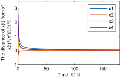
Figure 2. Image of the distance between the solved and the minimum point over time
图2. 所求解与最小值点之间的距离随时间变化图像
6. 结论
目前常用SAA方法求解有约束随机优化问题,但其计算较为复杂。通过上述数值模拟可以发现,本文提出的二阶微分方程方法求解例5.1和例5.2的速度较快,精度较小,并且所求的结果能够较为平滑的收敛到最优解。因此,二阶微分方程方法在求解等式约束随机优化问题时是收敛的。
但本文只验证了二阶微分方程算法可以求解等式约束下的随机优化问题,对于求解不等式约束的随机优化问题和随机约束的随机优化问题,二阶微分方程方法是否也具有良好的收敛性,值得下一步的探讨和研究。
文章引用
吕琪楠,孙菊贺,王 莉,谢红俭. 求解具有等式约束的随机优化问题的二阶微分方程方法
Second Order Differential Equation Algorithm for Solving Stochastic Optimization Problems with Equality Constraints[J]. 应用数学进展, 2023, 12(10): 4529-4537. https://doi.org/10.12677/AAM.2023.1210444
参考文献
- 1. Ferguson, A.R. and Dantzig, G.B. (1956) The Allocation of Aircraft to Routes—An Example of Linear Programming under Uncertain Demand. Management Science, 3, 45-73. https://doi.org/10.1287/mnsc.3.1.45
- 2. Dantzig, G.B. (2004) Linear Programming under Uncertainty. Management Science, 50, 1764-1769. https://doi.org/10.1287/mnsc.1040.0261
- 3. Kiefer, J. and Wolfowitz, J. (1952) Stochastic Estimation of the Maximum of a Regression Function. The Annals of Mathematical Statistics, 23, 462-466. https://doi.org/10.1214/aoms/1177729392
- 4. Spall, J.C. (1992) Multivariate Stochastic Approximation Using a Simultaneous Perturbation Gradient Approximation. IEEE Transactions on Automatic Control, 37, 332-341. https://doi.org/10.1109/9.119632
- 5. Chen, R., Menickelly, M. and Scheinberg, K. (2018) Stochastic Optimization Using a Trust-Region Method and Random Models. Mathematical Programming, 169, 447-487. https://doi.org/10.1007/s10107-017-1141-8
- 6. Billups, S.C., Graf, P. and Larson, J. (2013) Derivative-Free Optimization of Expensive Functions with Computational Error Using Weighted Regression. SIAM Journal on Optimization, 23, 27-53. https://doi.org/10.1137/100814688
- 7. Guo, J.H., Liu, H.L. and Xiao, X.T. (2020) A Unified Analysis of Stochastic Gradient-Free Frank-Wolfe Methods. International Transactions in Operational Research, 29, 63-86. https://doi.org/10.1111/itor.12889
- 8. Curtis, F.E., Scheinberg, K. and Shi, R. (2017) A Stochastic Trust Region Algorithm. Industrial and Systems Engineering, 1-16.
- 9. Schmidt, M., Roux, N.L. and Bach, F. (2017) Minimizing Finite Sums with the Stochastic Average Gradient. Mathematical Programming, 162, 83-112. https://doi.org/10.1007/s10107-016-1030-6
- 10. Nie, Y.Y. (2013) Convergence Theory of a SAA Method for Min-Max Stochastic Optimization Problems. Applied Mechanics and Materials, 303-306, 1319-1322. https://doi.org/10.4028/www.scientific.net/AMM.303-306.1319
- 11. Ghadimi, S. and Lan, G. (2016) Accelerated Gradient Methods for Nonconvex Nonlinear and Stochastic Programming. Mathematical Programming, 156, 59-99. https://doi.org/10.1007/s10107-015-0871-8
- 12. Chen, X.J., Qi, L. and Womersley, R.S. (1995) Newton’s Method for Quadratic Stochastic Programs with Recourse. Journal of Computational and Applied Mathematics, 60, 29-46. https://doi.org/10.1016/0377-0427(94)00082-C
- 13. Nemirovski, A., Juditsky, A., Lan, G., et al. (2009) Robust Stochastic Approximation Approach to Stochastic Programming. SIAM Journal on Optimization, 19, 1574-1609. https://doi.org/10.1137/070704277
- 14. Qu, X. and Bian, W. (2022) Fast Inertial Dynamic Algorithm with Smoothing Method for Nonsmooth Convex Optimization. Computational Optimization and Applications, 3, 287-317. https://doi.org/10.1007/s10589-022-00388-6
- 15. Polyak, B.T. and Juditsky, A.B. (1992) Acceleration of Stochastic Approximation by Averaging. SIAM Journal on Control and Optimization, 30, 838-855. https://doi.org/10.1137/0330046