Advances in Applied Mathematics
Vol.07 No.06(2018), Article ID:25479,5
pages
10.12677/AAM.2018.76081
Hopf Bifurcation in a Class of Predator-Prey Systems
Zizun Li
School of Mathematics and Statistics, Baise University, Baise Guangxi

Received: May 24th, 2018; accepted: Jun. 12th, 2018; published: Jun. 19th, 2018

ABSTRACT
In this paper, we studied a class of predator-prey system with a defense mechanism of the prey. By calculating the Lyapunov coefficient, the internal equilibrium point is proved to be a first order weak focus, and the parameter conditions of Hopf bifurcation are given.
Keywords:Predator-Prey System, Lyapunov Coefficient, Hopf Bifurcation
一类捕食系统中的Hopf分岔
李自尊
百色学院,广西 百色
收稿日期:2018年5月24日;录用日期:2018年6月12日;发布日期:2018年6月19日

摘 要
本文研究了食饵具有防御机制的一类捕食系统。通过计算Lyapunov系数证明内部平衡点为一阶细焦点, 并给出了Hopf分岔的参数条件。
关键词 :捕食系统,Lyapunov系数,Hopf分岔

Copyright © 2018 by author and Hans Publishers Inc.
This work is licensed under the Creative Commons Attribution International License (CC BY).
http://creativecommons.org/licenses/by/4.0/


1. 引言
Ajraldi [1] 研究了如下的食饵具有牧群行为的广义Holling-II功能函数反应
Braza [2] 研究了简化的食饵含有二次根号防御机制的函数反应
给出了内部平衡定的稳定性分析,在给出Hopf分岔分析时,并未计算Lyapunov系数,所以并不清楚在Hopf临界值时细焦点的阶数。
本文在上述研究成果的基础上,研究了一类食饵具有三次根号防御机制的函数反应
(1)
给出了内部平衡点的稳定性分析,并在判断Hopf分岔时给出了Lyapunov系数的值,计算出平衡点的类型为一阶稳定细焦点,改变参数后系统会发生Hopf分岔,平衡点的稳定性改变,分岔出一个稳定的极限环(参考 [3] [4] [5] )。
2. 主要结果
方程(1)的内部平衡点为 ,其Jacobian矩阵为
(2)
定理2.1 假设 ,即为 ,则系统(1)在 有一个从平衡点E经过
Hopf分岔出的稳定的极限环。
证明 由(2),可得
(3)
令 。
由(3),可得
当 时, ,可得
我们可以检验如下横截条件
在 时,平衡点 的坐标为
为了把平衡点坐标移到原点 ,我们作平移变换
则系统(1)变换为
(4)
我们可以把系统(4)写成如下形式
其中B,C为向量函数,令 ,则由(4),可得
(5)
(6)
其中 ,即为
(7)
其中 。
方程 的复特征向量为
(8)
且 。由(5),(6),(8)可得
(9)
且
(10)
由(8),(9),(10),可得
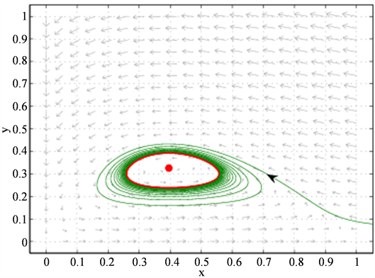
Figure 1. Stable limit cycle phase diagram of bifurcation from equilibrium point, bifurcation parameter is
图1. 从平衡点 分岔出的稳定的极限环相图,其中分岔参数为
我们可以计算参数在 时的平衡点E的第一Lyapunov系数为
则 为一阶细焦点,所以,当 时,从平衡点 分岔出一个稳定的极限环,参看图1。
基金项目
国家自然科学基金项目(11561019);中央高校基本科研业务费专项资金资助(2012017yjsy141)。
文章引用
李自尊. 一类捕食系统中的Hopf分岔
Hopf Bifurcation in a Class of Predator-Prey Systems[J]. 应用数学进展, 2018, 07(06): 680-684. https://doi.org/10.12677/AAM.2018.76081
参考文献
- 1. Ajraldi, V., Pittavino, M. and Venturino, E. (2011) Modeling Herd Behavior in Population Systems. Nonlinear Analysis: Real World Applications, 12, 2319-2338.
https://doi.org/10.1016/j.nonrwa.2011.02.002 - 2. Braza, P.A. (2012) Predator-Prey Dynamics with Square Root Functional Responses. Nonlinear Analysis: Real World Applications, 13, 1837-1843.
https://doi.org/10.1016/j.nonrwa.2011.12.014 - 3. Kuznetsov, Y.A. (2004) Elements of Applied Bifurcation Theory. Spring-er-Verlag, New York.
https://doi.org/10.1007/978-1-4757-3978-7 - 4. 张芷芬, 丁同仁, 黄文灶, 董镇喜, 微分方程定性理论[M]. 北京: 科学出版社, 1981.
- 5. 张伟年, 杜正东, 徐冰, 常微分方程[M]. 北京: 高等教育出版社, 2006.