Open Journal of Acoustics and Vibration
Vol.
07
No.
04
(
2019
), Article ID:
33565
,
8
pages
10.12677/OJAV.2019.74020
Acoustic Analysis Based on Isogeometric Boundary Element Method with Subdivision Surfaces
Yangyang Yan, Yu Zhang, Leilei Chen
College of Architecture and Civil Engineering, Xinyang Normal University, Xinyang Henan
![]()
Received: Dec. 3rd, 2019; accepted: Dec. 16th, 2019; published: Dec. 23rd, 2019

ABSTRACT
The core idea of subdivision surfaces is to repeatedly refine the initial polygon mesh and obtain smooth limit surfaces. The Catmull-Clark subdivision surface is developed based on the bicubic B-spline and is suitable for subdivision and fitting operations on arbitrary quadrilateral meshes. Combining the subdivision surface with the boundary element method, spline interpolation is applied to both geometry and physics in numerical analysis, which ensures the geometric accuracy of the analysis model and improves the accuracy of physical interpolation. In this paper, a Catmull-Clark based on subdivision surface method and a Catmull-Clark based on acoustic boundary element method are used to establish an extremely smooth spherical model, and the model is used to analyze the acoustic scattering response when plane waves are incident to prove the accuracy of the CCBEM method.
Keywords:Subdivision Surfaces, Boundary Element Method, Acoustic Scattering

基于细分曲面边界元法的声学分析
闫洋洋,张雨,陈磊磊
信阳师范学院建筑与土木工程学院,河南 信阳

收稿日期:2019年12月3日;录用日期:2019年12月16日;发布日期:2019年12月23日

摘 要
细分曲面核心思想是通过对初始多边形网格进行重复细化,并得到光滑极限曲面。Catmull-Clark细分曲面是基于双三次B样条发展起来的,适用于对任意四边形网格进行细分和拟合操作。将细分曲面与边界元法结合起来,在数值分析中几何与物理都采用样条插值,保证了分析模型的几何精确性,同时也使物理插值的精度有所提高。本文通过联合基于Catmull-Clark的细分曲面法和声学边界元法,建立极限光滑球形模型,并用此模型分析在平面波入射时球模型表面的声散射响应,以证明CCBEM (Catmull-Clark边界元法)方法的正确性。
关键词 :细分曲面,边界元法,声散射

Copyright © 2019 by author(s) and Hans Publishers Inc.
This work is licensed under the Creative Commons Attribution International License (CC BY).
http://creativecommons.org/licenses/by/4.0/


1. 引言
相比于NURBS (非均匀有理B样条)建模,细分曲面建模的数值更为稳定,更易实现,并且适用于任意拓扑结构。细分曲面的基本思想是对初始多边形网格重复细化,最终拟合为光滑曲面。细分曲面的概念简单,不需要对算法做重大改变,便很容易被修改 [1]。细分曲面广泛地应用在声学、电磁学、计算机制图、3D打印、动画和游戏等领域。
边界元法的实质是只对定义域的边界离散,而不需要对域内离散,具有计算精度高和数据准备简单的优点 [2]。用边界元法求解非线性问题时,会遇到同非线性项所对应的区域积分,这种积分在奇异点周围有强烈的奇异性,因而求解过程存在困难 [3]。
将细分曲面和边界元法结合,能根据不同精度对细分层级网格的要求做相应的调整,省去前处理中模型的重复离散过程。本文介绍了基于Catmull-Clark的细分曲面方法和基于Catmull-Clark的声学边界元法的详细计算过程,此外,通过分析散射球模型在平面波入射的声散射响应,以及散射球内某点的散射声压分布情况,证明CCBEM算法的有效性和正确性。本文创新性地将CBIE (传统单边界积分方程)和组合Burton-Miller边界积分方程应用于散射球模型的数值计算中,并比较两种方法在数值计算中的优缺点,发现基于CBIE的数值结果在某些频率上偏离解析解,但基于组合Burton-Miller边界积分方程的结果和解析解几乎一致。
2. 基于Catmull-Clark的细分曲面方法
2.1. Catmull-Clark细分规则
CC (Catmull-Clark)是将任意四边形网格细分为四个子四边形网格的算法 [4]。k级网格细分一次生成三种顶点:1、原始网格根据周围顶点权重获得顶点V;2、在任意四边形单元的各边的中部插入E顶点;3、在任意四边形单元的中心位置插入F顶点。三顶点的计算表达式如下 [5] :(如图1所示)
1) 顶点坐标为:
(1)
,,, 和 为相邻顶点坐标。
2) 顶点坐标为:
(2)
,,,,, 为相邻顶点的坐标。
3) 顶点坐标为:
(3)
,,, 为四边形单元的坐标。

Figure 1. Distribution of edge point “E”, midpoint “F” and vertex point “V”
图1. 边点E和顶点V的分布
2.2. 曲面拟合
2.2.1. 规则单元曲面拟合
规则四边形单元曲面拟合时,拟合单元内某点的局部参数坐标为 。该点的笛卡尔坐标 为 [6] :
(4)
为第i个相邻顶点的坐标,参数域满足 , 为双三次B样条基函数
(5)
为余数, 为除法,N为三次B样条基函数
(6)
(7)
(8)
(9)
2.2.2. 不规则单元的曲面拟合
对于不规则单元的曲面拟合,拟合点坐标为 [7] :
(10)
为拾取矩阵, 为初始拟合点x的坐标, 为细分后规则子单元中拟合点x的坐标。
规则单元中,拟合点的笛卡尔坐标 为
(11)
是第i个相邻顶点的坐标, 是不规则单元的基函数, 是基函数矩阵
(12)
3. 基于Catmull-Clark的声学边界元法
3.1. 声学边界积分公式
控制声域的赫姆霍兹方程为
(13)
为拉普拉斯算子, 为点x处的声压,波数为 , 为角频率,c为传播流体域中的声波速度。对公式(13)进行一系列转换后,可以得到以下边界积分方程
(14)
为入射波声压, 和v为边界积分算子。
对公式(14)求法向导数积分方程,可得积分方程 [8] :
(15)
在外边界值问题中,公式(14)和(15)单独使用时,方程式存在虚拟特征频率。但是,这两个方程的线性组合可以克服该问题,对于如何克服虚拟特征频率的详细过程,可参考 [9] 表示如下
(16)
为组合参数:当 时, ,否则 。
3.2. 离散化
首先,用CC细分单元离散边界,再用物理场近似每个单元,
(17)
、 为 单元内点 的声压、法线通量, 、 为 单元网格中某节点的声压、法线通量。
(18)
通过使方程式(18)保持在选定的搭配点上,并集合这些公式,可以得到以下等式,
(19)
H、G是CCBEM的系数矩阵,p、 是配置点处的声压和入射波矩阵。
4. 数值例子
散射球
对于具有解析解的半径为5的散射球,本文给出初始粗糙离散四边形模型,然后对其连续细分操作,以观察每个细分层次,如图2所示。从图2可知,散射球模型中存在的不规则点,不会随细分次数的增加而变化,规则点随细分次数,成指数形式增长。
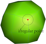 (a) 初始网格
 (b) 1级细分网格
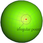 (c) 2级细分网格
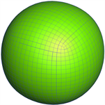 (d) 3级细分网格
 (e) 4级细分网格
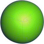
 (f) 极限细分网格
Figure 2. Initial mesh and multilevel subdivision meshes: (a) initial mesh with 24 elements and 26 nodes; (b) 1 level of subdivision surface with 98 nodes and 96 elements; (c) 2 level of subdivision surface with 386 nodes and 384 elements; (d) 3 level of subdivision surface with 1538 nodes and 1536 elements; (e) 4 level of subdivision surface with 6146 nodes and 6144 elements; (f) limited subdivision surface with 98,306 nodes and 98,304 element
图2. 初始网格和多级细分网格:(a) 有24个单元和26个节点的初始网格;(b) 1级细分曲面,有98个节点和96个单元;(c) 有386个节点和384个单元的2级细分曲面;(d) 有1538个节点和1536个单元的3级细分曲面;(e) 有6146个节点和6144个单元的4级细分曲面;(f) 极限细分曲面,有98,306个节点和98,304个单元
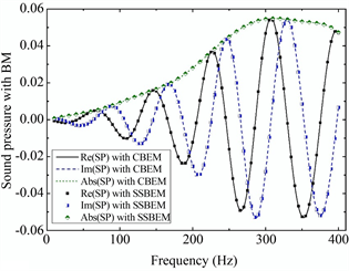
构建光滑球形模型后,本文分析了极限球形模型在平面波入射时的声散射响应,以证明CCBEM方法的正确性。平面波沿X轴正向传播,幅度为1。本文研究了点 处频率的散射声压,如图3所示。CBIE和组合Burton-Miller边界积分方程用于数值计算。由图4可知,基于CBIE方程的数值结果在某些频率上偏离解析解,但是基于组合方程的结果和解析解几乎一致。这是BEM(边界元法)方法在解决外部声学问题时的一个特殊问题,但不是分析模型时存在的固有问题。若模型在某频率上无法得到正确结果,则该频率称为虚拟特征频率。此外,图4还验证了在本文中得以发展的CCBEM算法的正确性。
如图3所示,相同的极限光滑模型用于多频响应分析。从图4可知CBIE的结果在几个虚拟频率上迅速振荡。随着频率越来越高,模型中虚拟频率的分布越来越密集。但是,组合方程的结果在整个频率带上都非常平缓。
 (a) 实部
 (b) 虚部
Figure 3. Comparisons between numerical and analytical solutions of sound pressure at a point of (10;0;0): (a) Real part of sound pressure as a function of frequency; (b) Imaginary part of sound pressure as a function of frequency. The frequency step is 0.1 Hz
图3. 点(10;0;0)处声压的数值解和解析解两者之间的比较:(a) 声压随频率变化的实部;(b) 声压随频率变化的虚部。频率步距为0.1 Hz
 (a) CBIE的声压
 (b) BM的声压
Figure 4. Changes in the real, imaginary, and amplitude of the sound pressure at point (2; 0; 0) with frequency: (a) CBIE is used for numerial solution; (b) BM is used for numerial solution. Black solid line denotes the real part of sound pressure with CBEM; Dash line denotes the imaginary part of sound pressure with CBEM; Dot line denotes the amplitute of sound pressure with CBEM; Three different types of scatters are used to represent the solution by CCBEM
图4. 点(2;0;0)处的声压的实部,虚部和幅度随频率的变化情况:(a)CBIE用于数值解;(b)BM用于数值解。黑色实线代表CBEM(传统边界元法)的声压的实部;虚线代表CBEM的声压的虚部;CCBEM使用三种不同类型的散射来表示解决方案
对于虚拟频率的分布情况,可由以下计算过程得知:
在Neumann边值条件下:
若边界径向速度给定为 ,则系数A满足 [10]
(20)
可得
(21)
则对应内域声场问题的特解为
(22)
由上式可知,Neumann边值条件的内域声场问题的特征波数为使 的k值,即满足 。由上述计算过程可知,对于脉动球算例,常规边界积分方程的非唯一解出现在 处。
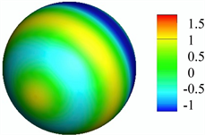
图5显示了两个频率上,极限光滑球形曲面上的声压的实部、虚部,以及曲面误差的分布。并且,从图5可知,图形具有良好的轴对称性。极限球两端的误差很小,但中部的误差很大。另外,频率越大,极限球面上的误差越大。
 (a) 50 HZ时的实部
 (b) 50 HZ时的虚部
 (c) 50 HZ时的曲面误差
![]() (d) 100 HZ时的实部
(d) 100 HZ时的实部
![]() (e) 100 HZ时的虚部
(e) 100 HZ时的虚部
![]() (f) 100 HZ时的曲面误差
(f) 100 HZ时的曲面误差
Figure 5. Distribution of sound pressure and surface error on limited spherical surface:(a) Real part of sound pressure at 50 Hz; (b) Imaginary part of sound pressure at 50 Hz; (c) Surface error at 50 Hz; (d) Real part of sound pressure at 100 Hz; (e) Imaginary part of sound pressure at 100 Hz;(f) Surface error at 100 Hz
图5. 极限球面上的声压和曲面误差的分布:(a) 50 Hz时声压的实部;(b) 50 Hz时声压的虚部;(c) 50 Hz时的曲面误差;(d) 100 Hz时声压的实部;(e) 100 Hz时声压的虚部;(f)100 Hz时的曲面误差
5. 总结
本文用基于CC的细分曲面法和基于CC的声学边界元法,研究了散射球在平面波入射时的声散射响应,从而验证了CCBEM的正确性和有效性,并发现球模型中存在的不规则点,不会随细分次数的改变而改变,基于CBIE方程的数值结果在某些频率上偏离解析解,但基于组合Burton-Miller边界积分方程的计算结果和解析解几乎一致。
文章引用
闫洋洋,张 雨,陈磊磊. 基于细分曲面边界元法的声学分析
Acoustic Analysis Based on Isogeometric Boundary Element Method with Subdivision Surfaces[J]. 声学与振动, 2019, 07(04): 175-182. https://doi.org/10.12677/OJAV.2019.74020
参考文献
- 1. Pan, Q., Xu, G.L. and Zhang, Y.J. (2013) A Unified Method for Hybrid Subdivision Surface Design Using Geometric Partial Differential Equations. Computer-Aided Design, 46, 110-119. https://doi.org/10.1016/j.cad.2013.08.023
- 2. Hughes, T., Reali, A. and Sangalli, G. (2010) Efficient Quadrature for NURBS-Based Isogeometric Analysis. Computer Methods in Applied Mechanics and Engineering, 199, 301-313. https://doi.org/10.1016/j.cma.2008.12.004
- 3. Jüttler, B., Mantzaflaris, A., Perl, R. and Rumpf, M. (2016) On Numer-ical Integration in Isogeometric Subdivision Methods for PDEs on Surfaces. Computer Methods in Applied Mechanics and Engineering, 302, 131-146. https://doi.org/10.1016/j.cma.2016.01.005
- 4. Shen, J.J., Kosinka, J., Sabin, M. and Dodgson, N. (2014) Conversion of Trimmed NURBS Surfaces to Catmull-Clark Subdivision Surfaces. Computer Aided Geometric Design, 31, 486-498. https://doi.org/10.1016/j.cagd.2014.06.004
- 5. Wawrzinek, A. and Polthier, K. (2016) Integration of Generalized B-Spline Functions on Catmull-Clark Surfaces at Singularities. Computer-Aided Design, 78, 60-70. https://doi.org/10.1016/j.cad.2016.05.008
- 6. Wei, X.D., Zhang, Y.J., Hughes, T.J.R. and Scott, M.A. (2015) Trun-cated Hierarchical Catmull-Clark Subdivision with Local Refinement. Computer Methods in Applied Mechanics and En-gineering, 291, 1-20. https://doi.org/10.1016/j.cma.2015.03.019
- 7. Pan, Q., Xu, G.L., Xu, G. and Zhang, Y.J. (2016) Isogeometric Analy-sis Based on Extended Catmull-Clark Subdivision. Computers and Mathematics with Applications, 71, 105-119. https://doi.org/10.1016/j.camwa.2015.11.012
- 8. Oden, J.T., Prudhomme, S. and Demkowicz, L. (2005) A Posteriori Error Estimation for Acoustic Wave Propagation Problems. Archives of Computational Methods in Engineering, 12, 343-389. https://doi.org/10.1007/BF02736190
- 9. Chen, L., Zheng, C. and Chen, H. (2014) FEM/Wideband FMBEM Coupling for Structural-Acoustic Design Sensitivity Analysis. Computer Methods in Applied Mechanics and Engineer-ing, 276, 1-19. https://doi.org/10.1016/j.cma.2014.03.016
- 10. 郑昌军. 三维结构声学及其敏感度分析的宽度快速多级边界元算法研究[D]: [博士学位论文]. 合肥: 中国科学技术大学, 2011.