一类耦合Burgers方程组的数值计算 Numerical Solution to Coupled Burgers’ Equations

doi:10.12677/AAM.2019.812225

Advances in Applied Mathematics
Vol. 08 No. 12 ( 2019 ), Article ID: 33379 , 12 pages
10.12677/AAM.2019.812225

Numerical Solution to Coupled Burgers’ Equations

Le Su, Wei Gao

●How to Cite this Article

School of Mathematical Sciences, Inner Mongolia University, Hohhot Inner Mongolia

Received: Nov. 15^th, 2019; accepted: Dec. 3^rd, 2019; published: Dec. 10^th, 2019

ABSTRACT

This paper solves a class of coupled Burgers’ equations based on finite volume scheme in a uniform grid. A new scheme for discretizing convective term is constructed by Hermite interpolation method with satisfying TVD (Total Variational Diminishing) criterion, and the time discretization is fulfilled by using the third-order Runge-Kutta scheme. It is verified that this scheme has gained a good computational performance by several classical numerical examples.

Keywords:Coupled Burgers’ System, Finite Volume Method, Discrete

一类耦合Burgers方程组的数值计算

宿乐，高巍

内蒙古大学数学科学学院，内蒙古呼和浩特

收稿日期：2019年11月15日；录用日期：2019年12月3日；发布日期：2019年12月10日

摘要

本文基于有限体积格式，对于一类耦合Burgers方程组问题，在满足TVD (Total Variational Diminishing)准则的情况下，利用Hermite插值法建立了新的格式离散对流项，并利用三阶Runge-Kutta格式对时间项进行离散，通过经典的数值算例验证，该格式具有良好的计算效果。

关键词 :耦合Burgers方程组，有限体积法，离散

This work is licensed under the Creative Commons Attribution International License (CC BY).

http://creativecommons.org/licenses/by/4.0/

1. 引言

众所周知，非线性耦合Burgers方程不具有精确的解析解。但由于其在科学和工程领域的广泛适用性，科学家和专家们对利用各种数值技术研究Burgers方程的性质很感兴趣。

一类耦合Burgers方程组：

$\frac{\partial u}{\partial t} - δ \frac{\partial^{2} u}{\partial x^{2}} + η u \frac{\partial u}{\partial x} + α \frac{\partial (u v)}{\partial x} = 0, x \in Ω = [a, b], t \in [0, T]$

$\frac{\partial v}{\partial t} - μ \frac{\partial^{2} v}{\partial x^{2}} + ξ v \frac{\partial v}{\partial x} + β \frac{\partial (u v)}{\partial x} = 0, x \in Ω = [a, b], t \in [0, T]$

初值条件：

$u (x, 0) = g_{1} (x), x \in Ω = [a, b]$

$v (x, 0) = g_{2} (x), x \in Ω = [a, b]$

边界条件：

$u (a, t) = f_{1} (t), u (b, t) = f_{2} (t), t \in [0, T]$

$v (a, t) = f_{3} (t), v (b, t) = f_{4} (t), t \in [0, T]$

其中 $δ$ ， $μ$ ， $η$ ， $ξ$ 是实常数， $α$ ， $β$ 是任意常数，取决于系统参数。 $u (x, t)$ 和 $v (x, t)$ 是待测定的速度分量。 $\frac{\partial u}{\partial t}$ 为非定常项， $u (\frac{\partial u}{\partial x})$ 为非线性对流项， $\frac{\partial^{2} u}{\partial x^{2}}$ 为扩散项。 $g_{1} (x)$ ， $g_{2} (x)$ ， $f_{1} (t)$ ， $f_{2} (t)$ ， $f_{3} (t)$ ， $f_{4} (t)$ 是充分光滑函数。

Esipov [1] 推导了一维粘性Burgers方程，研究了多分散沉降模型。该耦合方程是重力作用下两种颗粒在流体悬浮液或胶体中的沉降或单位体积浓度(scaled volume concentrations)演化的简单模型。Burgers [2] 和Cole [3] 发现，该方程组描述了各种现象，如湍流的数学模型和在粘性流体中流过激波的近似理论。Soliman [4] 采用了改进的扩展的Tanh函数法得出一维耦合Burgers分解法的精确解，但在一般情况下，耦合burgers方程的解析解是不可用的。很多研究人员对一维耦合Burgers方程的数值解进行了求解。 Esipov给出了一些数值模拟，并将结果与实验数据进行了比较。Abdou和Soliman [5] 用变分迭代法求解一维Burgers方程和耦合Burgers方程。Deghan [6] 等人利用Adomian-Pade技术，得到了粘性Burgers耦合方程的数值结果。Mittal和Arora [7] 提出了一种基于Crank-Nicolson和三次B样条函数格式的耦合Burgers方程数值求解方法。Khater [8] 等提出了非线性偏微分方程近似解的Chebyshev谱配置法，利用Chebyshev谱配点法，将问题简化为一个ODES系统，然后用四阶Runge-Kutta方法求解。Rashid和Ismail [9] 等人利用空间上的Fourier伪谱法和经典的四阶Runge-Kutta方法，给出了具有一组初值、周期边界条件的耦合Burgers方程的近似解。Mittal [10] 等人用多项式微分求积法(PDQM)分析了一个耦合Burgers方程。PDQM将耦合Burgers方程转化为非线性方程组，然后用四阶Runge-Kutta方法求解。Mohanty [11] 等人提出了一种求解耦合Burgers方程的四阶隐式紧算子方法，没有使用任何变换或线性化技术来处理非线性项。Arminjon和Beuchamp [12] 提出了二维耦合Burgers方程的有限元方法，并得出了与其他方法，即直线法和Runge-Kutta型方法相比，该方法是有效的。魏 [13] 等人提出了空间离散的分布式逼近泛函格式和求解一维和二维Burgers方程的Taylor级数展开方法。

本文采用有限体积法对耦合Burgers方程组进行求解，有限体积法在离散化之前不需要对非线性项进行线性化处理，用有限体积法得到的离散方程，可以完美地体现守恒性。最后，将经该格式计算后的数值解和文献 [7] [14] [15] [16] [17] 中已有的精确解进行了比较，发现计算结果较好。

本论文以QUICK有限体积格式为基础，构造了一个满足TVD和CBC-BAIR约束条件的高阶有界有限体积数值格式，用于计算耦合Burgers方程组的数值解。本文的安排具体如下：第一章是引言；第二章建立了对流项的高分辨率有限体积格式和扩散项的数值离散；第三章以典型的耦合Burgers方程组为例，给出了几个的数值算例；第四章给出了结论。

2. 数值格式的构建

2.1. Burgers方程

以Burgers方程为例：

$\frac{\partial u}{\partial t} + u \frac{\partial u}{\partial x} = ν \frac{\partial^{2} u}{\partial x^{2}}, x \in Ω = [a, b], t \in [0, T]$ (2.1)

下利用有限体积法给出具体求解过程。

将计算区间 $[a, b]$ 剖分成N个等距的网格，记

$x_{\frac{1}{2}} = a < x_{\frac{3}{2}} = a + Δ x < \dots < x_{N + \frac{1}{2}} = b$ (2.2)

则有每一个控制单元 $I_{j} = [x_{j - \frac{1}{2}}, x_{j + \frac{1}{2}}], j = (1, \dots, N)$ 的长度为 $Δ x = \frac{b - a}{N}$

将(2.1)式在 $I_{j}$ 上积分，可得

$\int_{I_{j}} \frac{\partial u}{\partial t} d x + \int_{I_{j}} \frac{\partial f}{\partial x} d x = \int_{I_{j}} ν \frac{\partial^{2} u}{\partial x^{2}} d x$

其中， $f = u^{2}$ 。

进一步写成

$\frac{\partial}{\partial t} \int_{I_{j}} u (x, t) d x + {f (x, t) |}_{x_{j + \frac{1}{2}}}^{x_{j + \frac{1}{2}}} = {ν \frac{\partial^{2} u}{\partial x^{2}} |}_{x_{j + \frac{1}{2}}}^{x_{j + \frac{1}{2}}}$ (2.3)

进而可得

$\frac{\partial}{\partial t} \int_{I_{j}} u (x, t) d x + [f (x_{j + \frac{1}{2}}, t) - f (x_{j - \frac{1}{2}}, t)] = ν [u^{'} (x_{j + \frac{1}{2}}, t) - u^{'} (x_{j + \frac{1}{2}}, t)]$ (2.4)

定义

${\bar{u}}_{j} (t) = \frac{1}{Δ x} \int_{I_{j}} u (x, t) d x$

是第j个单元的单元平均值，则(2.4)式可以简化为

$Δ x \frac{\partial {\bar{u}}_{j} (t)}{\partial t} + [f (x_{j + \frac{1}{2}}, t) - f (x_{j - \frac{1}{2}}, t)] = ν [u^{'} (x_{j + \frac{1}{2}}, t) - u^{'} (x_{j + \frac{1}{2}}, t)]$

为了简单起见，记

$u (x_{j + \frac{1}{2}}, t) = u_{j + \frac{1}{2}}$

则有

$Δ x \frac{\partial {\bar{u}}_{j} (t)}{\partial t} + (f_{j + \frac{1}{2}} - f_{j - \frac{1}{2}}) = v ({u^{'}}_{j + \frac{1}{2}} - {u^{'}}_{j - \frac{1}{2}})$ (2.5)

再次，引入空间离散，在 $t = t_{0}$ 时，由上面单元积分平均值的定义，可以计算 ${\bar{u}}_{1}^{0}, {\bar{u}}_{2}^{0}, \dots, {\bar{u}}_{N}^{0}$ ，由等式(2.5)可知，要求解 $t = t_{1}$ 时的 ${\bar{u}}_{1}^{1}, {\bar{u}}_{2}^{1}, \dots, {\bar{u}}_{N}^{1}$ 的话，必须知道单元界面处的点值。

下用单元积分平均值表示单元界面处的点值 $u (x_{j + \frac{1}{2}}, t), j = (0, 1, \dots, N)$ ，然后利用数值格式实现用单

元积分平均值表示点值，代入方程(2.5)，得出便于求解的线性方程或线性方程组。由图1可知，由于是等距剖分，故令 $x_{C} = x_{j}$ ，由于对流项的离散产生的数值耗散比较大，所以先建立对流项的离散格式。

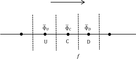
Figure 1. Three neighboring mesh points and the mesh face

图1. 三个相邻的节点及单元

2.2. 高阶格式

如图1所示，U、C、D是相邻的3个网格节点，分别表示上游(upwind point)、中心(central point)和下游(downwind point)的三个节点，f表示控制单元的界面(cell face)。若界面值 $ϕ_{f}$ 由单元平均值 $ϕ_{U}, ϕ_{C}, ϕ_{D}$ 确定，一般情况下，选取三个单元平均值重构界面值时可以表达成以下函数关系：

$ϕ_{f} = f ({\bar{ϕ}}_{U}, {\bar{ϕ}}_{C}, {\bar{ϕ}}_{D})$ (2.6)

则 $ϕ_{f}$ 可以表达为

$ϕ_{f} = {\bar{ϕ}}_{C} + [\frac{1 + k}{4} ({\bar{ϕ}}_{D} - {\bar{ϕ}}_{C}) + \frac{1 - k}{4} ({\bar{ϕ}}_{C} - {\bar{ϕ}}_{U})]$ (2.7)

其中，参数 $k \in [- 1, 1]$ ，对k赋不同的值可得到不同的高阶格式。根据Leonard的正则变量化方法 [18]，定义正则化变量形式(Normalized Variable Formulation, NVF)为

$\hat{ϕ} = \frac{\bar{ϕ} - {\bar{ϕ}}_{U}}{{\bar{ϕ}}_{D} - {\bar{ϕ}}_{U}}$

这里的 $ϕ$ 的取值为 $ϕ_{U}, ϕ_{C}, ϕ_{D}, ϕ_{f}$ 。于是有(2.6)的变量正则化形式是

${\hat{ϕ}}_{f} = f ({\hat{ϕ}}_{U}, {\hat{ϕ}}_{C}, {\hat{ϕ}}_{D})$ (2.8)

因为 ${\hat{ϕ}}_{U} = 0, {\hat{ϕ}}_{D} = 1$ ，所以(2.8)化简为

${\hat{ϕ}}_{f} = f ({\hat{ϕ}}_{C})$

则k格式(2.7)可化为

${\hat{ϕ}}_{f} = (1 - \frac{k}{2}) ϕ_{C} + \frac{1}{4} (1 + k)$ (2.9)

由式(2.9)得知， ${\hat{ϕ}}_{f}$ 的变化只依赖于k和 ${\hat{ϕ}}_{C}$ ，很大程度上简化了新的数值格式的建立过程。

表1给出了几种常见的对流格式的NV线，值得注意的是，这些线性高阶格式都不满足有界性，因此，采用有界性准则结合线性高阶格式来构造高分辨率格式。

Table 1. The linear convection schemes and the NV formulations

表1. 线性对流格式及其NV格式

通常称数值格式的正则变量化形式在 ${\hat{ϕ}}_{C} - {\hat{ϕ}}_{f}$ 坐标系上的图形表达为格式的正则变量图(Normalized Variable Diagram, NVD)，某一个格式在NVD上的图形表达称为其对应的NV线。在Leonard提出的NVD的基础上，Gaskell和Lau提出了对流有界性准则，即CBC准则。利用正则变量化形式，CBC准则可以表为：

${\begin{cases} {\hat{ϕ}}_{C} < {\hat{ϕ}}_{f} = f ({\hat{ϕ}}_{C}) < 1, 0 < {\hat{ϕ}}_{C} < 1 \\ {\hat{ϕ}}_{f} = {\hat{ϕ}}_{C}, {\hat{ϕ}}_{C} \leq 0 \\ {\hat{ϕ}}_{f} = {\hat{ϕ}}_{C}, {\hat{ϕ}}_{C} \geq 1 \end{cases}$ (2.10)

数值格式的有界性，又称单调性，是指其数值计算结果不会超过物理问题自身所规定的上下限，即网格界面值 $ϕ_{f}$ 应满足以下不等式：

$\min ({\hat{ϕ}}_{C}, {\hat{ϕ}}_{D}) \leq ϕ_{f} \leq \max ({\hat{ϕ}}_{C}, {\hat{ϕ}}_{D})$ (2.11)

现在来分析一下CBC准则是如何保证界面值满足有界性的。当 ${\hat{ϕ}}_{U} \leq {\hat{ϕ}}_{C} \leq {\hat{ϕ}}_{D}$ 或者 ${\hat{ϕ}}_{U} \geq {\hat{ϕ}}_{C} \geq {\hat{ϕ}}_{D}$ ，即解是单调时，此时如果界面值 $ϕ_{f}$ 满足

${\hat{ϕ}}_{C} \leq {\hat{ϕ}}_{f} \leq {\hat{ϕ}}_{D}$ 或者 ${\hat{ϕ}}_{C} \geq {\hat{ϕ}}_{f} \geq {\hat{ϕ}}_{D}$ (2.12)

${\hat{ϕ}}_{C} \leq {\hat{ϕ}}_{f} \leq 1$ ，当 $0 \leq {\hat{ϕ}}_{C} \leq 1$ (2.13)

当 ${\bar{ϕ}}_{C} \notin [{\bar{ϕ}}_{U}, {\bar{ϕ}}_{D}]$ 或者 ${\bar{ϕ}}_{C} \notin [{\bar{ϕ}}_{D}, {\bar{ϕ}}_{U}]$ 时，解不是单调的，此时如果使用一阶迎风格式 $ϕ_{f} = {\bar{ϕ}}_{C}$ ，就能保持解是单调的。上述情况用正则化变量形式表达就是

${\hat{ϕ}}_{f} = {\hat{ϕ}}_{C}$ ，当 ${\hat{ϕ}}_{C} < 0$ 或 ${\hat{ϕ}}_{C} > 1$ (2.14)

然而，Wei [19] 和Hou [20] 证明了CBC准则只能保证数值格式的有界性，而未提及数值格式的精度。为了克服这个缺点，Wei和Hou提出了一个改进的CBC准则，即BAIR准则。它的正则变量化形式为

${\begin{cases} \frac{3}{2} {\hat{ϕ}}_{C} \leq {\hat{ϕ}}_{f} = f ({\hat{ϕ}}_{C}) \leq \frac{1}{2} ({\hat{ϕ}}_{C} + 1), 0 < {\hat{ϕ}}_{C} < \frac{1}{2} \\ \frac{1}{2} ({\hat{ϕ}}_{C} + 1) \leq {\hat{ϕ}}_{f} \leq \frac{3}{2} {\hat{ϕ}}_{C} 且 {\hat{ϕ}}_{f} \leq 1, \frac{1}{2} \leq {\hat{ϕ}}_{C} \leq 1 \\ {\hat{ϕ}}_{f} = {\hat{ϕ}}_{C}, {\hat{ϕ}}_{C} \leq 0 或 {\hat{ϕ}}_{C} \geq 1 \end{cases}$ (2.15)

另一个重要的对流项有界性约束是TVD (Total Variational Diminishing)约束条件，用限制器函数表示为

$0 \leq ψ (r) \leq \min (2 r, 2), r > 0$

$ψ (r) = 0, r \leq 0$

其中 $ψ (r)$ 是一个限制器(limiter)函数，其中

$r = \frac{ϕ_{D} - ϕ_{C}}{ϕ_{C} - ϕ_{U}}$

TVD约束条件也可以表达为

${\begin{cases} {\hat{ϕ}}_{f} \leq 1 且 {\hat{ϕ}}_{f} \in [{\hat{ϕ}}_{C}, 2 {\hat{ϕ}}_{C}], 0 < {\hat{ϕ}}_{C} < 1 \\ {\hat{ϕ}}_{f} = {\hat{ϕ}}_{C}, {\hat{ϕ}}_{C} \leq 0 或 {\hat{ϕ}}_{C} \geq 1 \end{cases}$ (2.16)

综上所述，将BAIR区域与TVD区域绘制于图2中

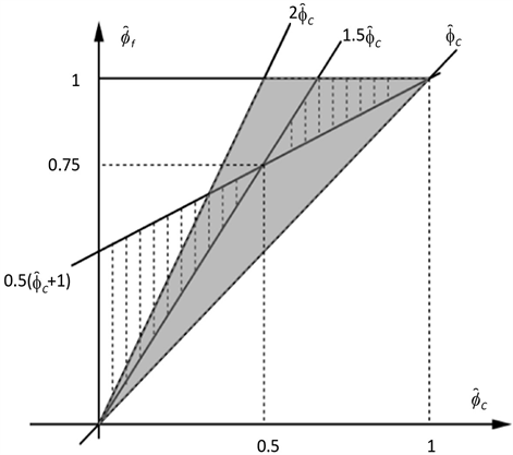
Figure 2. The regions of the TVD (shaded) and BAIR (hatched)

图2. BAIR区域(虚线部分)和TVD区域(阴影部分)

2.3. Hermite插值构造新格式

由上可知，若格式满足对流有界性，那么格式的NV线必须落在TVD区域和BAIR区域的重合区域内，由前面提到的HR格式的标准化形式： ${\hat{ϕ}}_{f} = f ({\hat{ϕ}}_{C})$ ，由图2可知

$f (0) = 0, f (\frac{1}{2}) = \frac{3}{4}, f (1) = 1$

由于所选的CUI格式不满足对流有界性，因此利用分段的思想来构造MCUI格式，使得此格式满足对流有界性准则。在 $\frac{1}{3} \leq {\hat{ϕ}}_{C} \leq \frac{2}{3}$ 的区间内，选取原有的CUI格式，在 $0 < {\hat{ϕ}}_{C} < \frac{1}{3}$ 内，选取 $f (0) = 0, f (\frac{1}{3}) = \frac{11}{18}$ 和 $f^{'} (0) = 2$ ，利用Hermite插值构造曲线，使曲线在重合的区域内，如图3所示，得到满足对流有界性的格式MCUI格式。该格式的正则化形式为

Figure 3. The illustration of the NV line of the MCUI scheme in the BAIR region

图3. MCUI格式在BAIR区域中的NV线

本文采用Local Lax-Friedrichs格式求解界面的数值通量f，任意单元体界面通量f可以表示为 $f = h (ϕ^{L}, ϕ^{R})$ ，利用Local Lax-Friedrichs计算数值流通量式子如下：

$f^{Lax} = \frac{1}{2} [f (ϕ^{L}) + f (ϕ^{R}) - \max | f^{'} (ϕ) | (ϕ^{R} - ϕ^{L})]$

对流项的离散完成后，扩散项采用二阶中心差分格式：

$\frac{\partial {\bar{φ}}_{j}}{\partial t} + \frac{1}{Δ x} ({\hat{f}}_{j + \frac{1}{2}} - {\hat{f}}_{j - \frac{1}{2}}) = \frac{v}{Δ x} (\frac{u_{j + 1} - 2 u_{j} + u_{j - 1}}{Δ x})$

2.4. 时间项的离散

完成了关于空间导数的离散后，得到了关于时间t的一个常微分方程，即

$\frac{d \bar{ϕ}}{d t} = L (ϕ)$

为了抑制非物理振荡，采用三阶Runge-Kutta格式进行离散：

${\begin{cases} ϕ^{(1)} = ϕ^{n} + L (ϕ^{n}) \\ ϕ^{(2)} = \frac{3}{4} ϕ^{n} + \frac{1}{4} [ϕ^{(1)} + L (ϕ^{(1)})] \\ ϕ^{n + 1} = \frac{1}{3} ϕ^{n} + \frac{2}{3} [ϕ^{(2)} + L (ϕ^{(2)})] \end{cases}$

3. 耦合Burgers方程组的数值算例

3.1. 算例1

对于耦合Burgers方程组

$\frac{\partial u}{\partial t} - δ \frac{\partial^{2} u}{\partial x^{2}} + η u \frac{\partial u}{\partial x} + α \frac{\partial (u v)}{\partial x} = 0, x \in Ω = [a, b], t \in [0, T]$

$\frac{\partial v}{\partial t} - μ \frac{\partial^{2} v}{\partial x^{2}} + ξ v \frac{\partial v}{\partial x} + β \frac{\partial (u v)}{\partial x} = 0, x \in Ω = [a, b], t \in [0, T]$

其中

$x \in [- π, π], δ = μ = 1.0, η = ξ = - 2.0, α = β = 1.0$

给定初边值条件：

$u (x, t) = v (x, t) = e^{- t} \sin (x)$

$u (0, t) = v (0, t) = \sin (x)$

分别计算 $u (x, t)$ ， $v (x, t)$ 在 $t = 0.0, 1.0, 2.0, 3.0$ 的数值解。

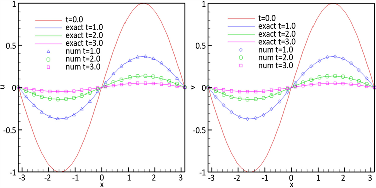
Figure 4. The numerical solution and the exact solution of Example 1 at different time for α = β = 1.0

图4. 算例1在不同时刻下的数值解和精确解，其中α = β = 1.0

经对比发现， $u (x, t)$ ， $v (x, t)$ 在不同时间数值解与精确解有很好的一致性。通过图4可以看出波的振幅随着时间的推移而减小，而波长保持不变。

3.2. 算例2

对于耦合Burgers方程组

$\frac{\partial u}{\partial t} - δ \frac{\partial^{2} u}{\partial x^{2}} + η u \frac{\partial u}{\partial x} + α \frac{\partial (u v)}{\partial x} = 0, x \in Ω = [a, b], t \in [0, T]$

$\frac{\partial v}{\partial t} - μ \frac{\partial^{2} v}{\partial x^{2}} + ξ v \frac{\partial v}{\partial x} + β \frac{\partial (u v)}{\partial x} = 0, x \in Ω = [a, b], t \in [0, T]$

给定初边值条件：

$u (x, t) = a_{0} - 2 A (\frac{2 α - 1}{4 α β - 1}) \tanh (A (x - 2 A t))$

$v (x, t) = a_{0} (\frac{2 β - 1}{2 α - 1}) - 2 A (\frac{2 α - 1}{4 α β - 1}) \tanh (A (x - 2 A t))$

$A = \frac{4 α β - 1}{4 α - 2}$

分别在以下三种情况下，计算 $u (x, t)$ ， $v (x, t)$ 在 $t = 1.0$ 时刻的数值解(见图5~7)：

情形1： $x \in [- 10, 10], δ = μ = 1.0, η = ξ = 2.0, α = 1.0, β = 2.0, a_{0} = 0.05$ ；

情形2： $x \in [- 10, 10], δ = μ = 1.0, η = ξ = 2.0, α = 0.1, β = 0.3, a_{0} = 0.05$ ；

情形3： $x \in [- 10, 10], δ = μ = 1.0, η = ξ = 2.0, α = 0.3, β = 0.03, a_{0} = 0.05$ 。

算例2的三组演化曲线以及 $u (x, t)$ ， $v (x, t)$ 在 $t = 0.5$ 和 $t = 1.0$ 的 $L_{2}$ 、 $L_{\infty}$ 误差表明，不同系数下， $u (x, t)$ ， $v (x, t)$ 的数值解对精确解的逼近效果较好(见表2和表3)。

Figure 5. The numerical solution and of Case 1 at t = 1.0 for α = 1.0, β = 2.0

图5. 情形1在t = 1.0时刻的数值解，其中α = 1.0, β = 2.0

Figure 6. The numerical solution and of Case 2 at t = 1.0 for α = 0.1, β = 0.3

图6. 情形2在t = 1.0时刻的数值解，其中α = 0.1, β = 0.3

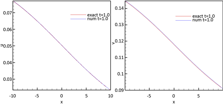
Figure 7. The numerical solution and of Case 3 at t = 1.0 for α = 0.3, β = 0.03

图7. 情形3在t = 1.0时刻的数值解，其中α = 0.3, β = 0.03

Table 2. Comparison of errors at different time for u(x,t) of Case 3

表2. 情形3中u(x,t)在不同时刻的误差比较

Table 3. Comparison of errors at different time for v(x,t) of Case 3

表3. 情形3中v(x,t)在不同时刻的误差比较

4. 结论

本文用有限体积法计算了一类耦合Burgers方程组的数值解，本文所采用的数值计算格式是基于BAIR准则和TVD准则，结合Hermite插值构造而成的。此格式简单方便，易于计算机实现。通过几个经典算例验证，此格式满足对流有界性、保持守恒特性，并且具有很好的计算效果。

基金项目

感谢内蒙古大学科研发展基金(21100-5187133)的支持。

文章引用

宿乐,高巍. 一类耦合Burgers方程组的数值计算
Numerical Solution to Coupled Burgers’ Equations[J]. 应用数学进展, 2019, 08(12): 1959-1970. https://doi.org/10.12677/AAM.2019.812225

参考文献

1. Esipov, S.E. (1995) Coupled Burgers’ Equations: A Model of Poly Dispersive Sedimentation. Physical Review E, 52, 3711-3718.
https://doi.org/10.1103/PhysRevE.52.3711

2. Burgers, M. (1948) A Mathematical Model Illustrating the Theory of Turbulence. Advances in Applied Mechanics, 1, 171-199.
https://doi.org/10.1016/S0065-2156(08)70100-5

3. Cole, D. (1951) On a Quasilinear Parabolic Equations Occurring in Aerodynamics. Quarterly of Applied Mathematics, 9, 225-236.
https://doi.org/10.1090/qam/42889

4. Soliman, A. (2006) The Modiﬁed Extended Tanh-Function Method for Solving Burgers-Type Equations. Physica A: Statistical Mechanics and Its Applications, 361, 394-404.
https://doi.org/10.1016/j.physa.2005.07.008

5. Abdou, M.A. and Soliman, A.A. (2005) Variational Iteration Method for Solving Burgers and Coupled Burgers Equations. Journal of Computational and Applied Mathematics, 181, 245-251.
https://doi.org/10.1016/j.cam.2004.11.032

6. Deghan, M., Asgar, H. and Mohammad, S. (2009) The Solution of Linear and Nonlinear Systems of Volterra Functional Equations Using Adomian-Pade Technique. Chaos, Solitons & Fractals, 39, 2509-2521.
https://doi.org/10.1016/j.chaos.2007.07.028

7. Mittal, R.C. and Arora, G. (2011) Numerical Solution of the Coupled Viscous Burgers’ Equation. Communications in Nonlinear Science and Numerical Simulation, 16, 1304-1313.
https://doi.org/10.1016/j.cnsns.2010.06.028

8. Khater, A.H., Temsah, R.S. and Hassan, M.M. (2008) A Chebyshev Spectral Collocation Method for Solving Burgers-Type Equations. Journal of Computational and Applied Mathematics, 222, 333-350.
https://doi.org/10.1016/j.cam.2007.11.007

9. Rashid, A. and Ismail, A. (2009) A Fourier Pseudo Spectral Method for Solving Coupled Viscous Burgers’ Equations. Computational Methods in Applied Mathematics, 9, 412-420.
https://doi.org/10.2478/cmam-2009-0026

10. Mittal, R.C. and Jiwari, R. (2012) Differential Quadrature Method for Numerical Solution of Coupled Viscous Burger’s Equation. International Journal for Computational Methods in Engineering Science and Mechanics, 13, 88-92.
https://doi.org/10.1080/15502287.2011.654175

11. Mohanty, R.K., Dai, W. and Han, F. (2015) Compact Operator Method of Accuracy Two in Time and Four in Space for the Numerical Solution of Coupled Viscous Burgers’ Equations. Applied Mathematics and Computation, 256, 381-393.
https://doi.org/10.1016/j.amc.2015.01.051

12. Arminjon, P. and Beauchamp, C. (1979) Numerical Solution of Burgers’ Equations in Two-Space Dimensions. Computer Methods in Applied Mechanics and Engineering, 19, 351-365.
https://doi.org/10.1016/0045-7825(79)90064-1

13. Wei, G.W., Zhang, D.S., Kouri, D.J. and Hoffman, D.K. (1998) Distributed Approximation Functional Approach to Burgers’ Equation in One and Two Space Dimensions. Computer Physics Communications, 111, 93-109.
https://doi.org/10.1016/S0010-4655(98)00041-1

14. Srivastava, V.K., Awasthi, M.K. and Tamsir, M. (2013) A Fully Implicit Finite-Difference Solution to One Dimensional Coupled Nonlinear Burgers’ Equations. International Journal of Mathematical, Computational Sciences and Engineering, 7, 283-287.
https://doi.org/10.1142/S1793557113500587

15. Rashida, A., Abbas, M., Izani, A. and Ismail, A.A.M. (2014) Numerical Solution of the Coupled Viscous Burgers Equations by Chebyshev-Legendre Pseudo-Spectral Method. Applied Mathematics and Computation, 245, 372-381.
https://doi.org/10.1016/j.amc.2014.07.067

16. Kumar, M. and Pandit, S. (2014) A Composite Numerical Scheme for the Numerical Simulation of Coupled Burgers’ Equation. Computer Physics Communications, 185, 809-817.
https://doi.org/10.1016/j.cpc.2013.11.012

17. Bhatt, H.P. and Khaliq, A.Q.M. (2016) Fourth-Order Compact Schemes for the Numerical Simulation of Coupled Burgers’ Equation. Computer Physics Communications, 200, 117-138.
https://doi.org/10.1016/j.cpc.2015.11.007

18. Leonard, B.P. (1988) Simple High-Accuracy Resolution Program for Convective Modeling of Discontinuities. International Journal for Numerical Methods in Fluids, 8, 1291-1318.
https://doi.org/10.1002/fld.1650081013

19. Wei, J.J., Yu, B. and Tao, W.Q. (2003) A New High-Order-Accurate and Bounded Scheme for Incompressible Flow. Numerical Heat Transfer, Part B: Fundamentals, 24, 353-337.

20. Hou, P.L. (2003) Refinement of the Convective Boundedness Criterion of Gaskell and Lau. Engineering Computations: International Journal for Computer-Aided Engineering, 20, 1023-1043.
https://doi.org/10.1108/02644400310503008

期刊菜单