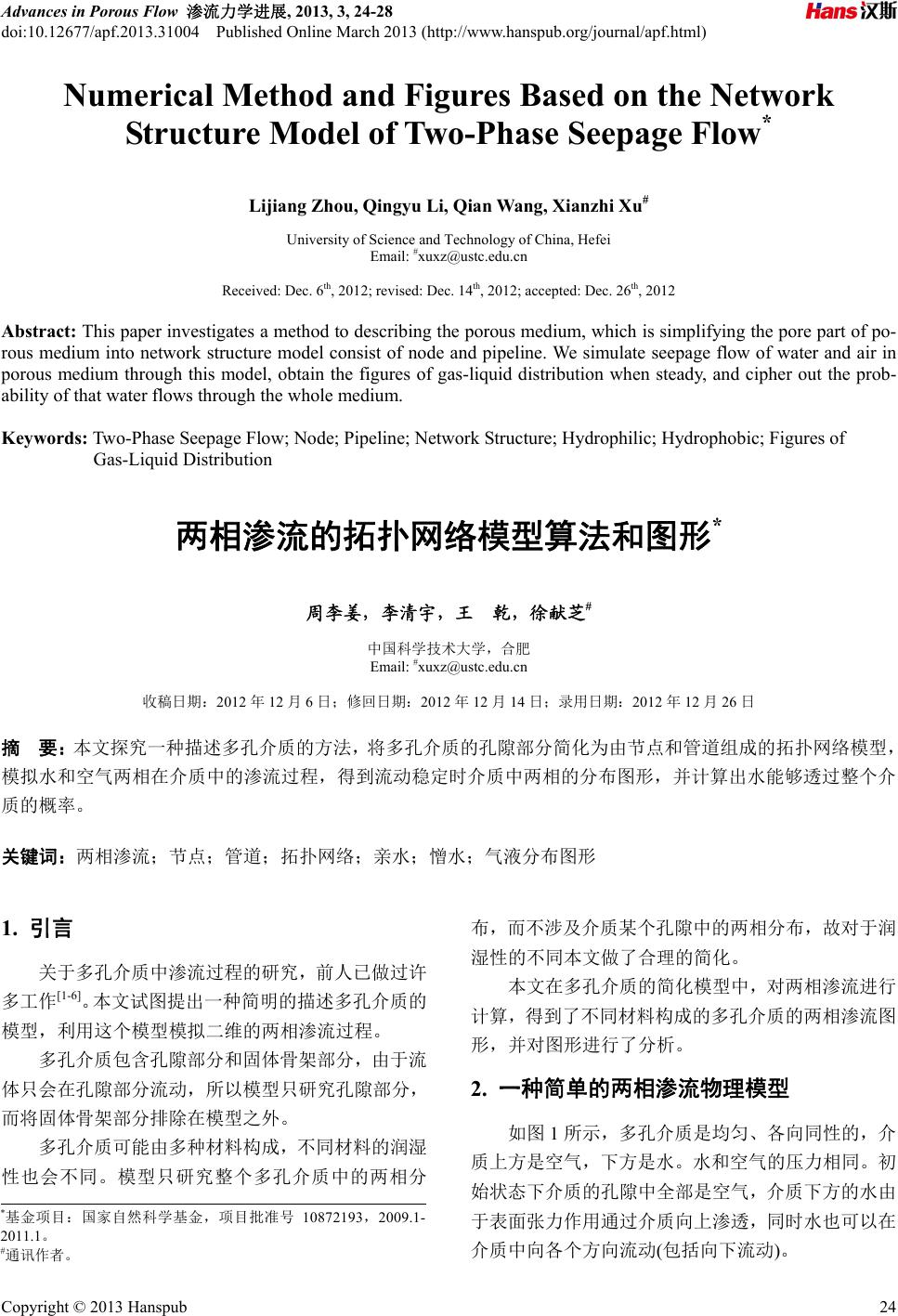
 Advances in Porous Flow 渗流力学进展, 2013, 3, 24-28 doi:10.12677/apf.2013.31004 Published Online March 2013 (http://www.hanspub.org/journal/apf.html) Copyright © 2013 Hanspub 24 Numerical Method and Figures Based on the Network Structure Model of Two-Phase Seepage Flow* Lijiang Zhou, Qingyu Li, Qian Wang, Xianzhi Xu# University of Science and Technology of China, Hefei Email: #xuxz@ustc.edu.cn Received: Dec. 6th, 2012; revised: Dec. 14th, 2012; accepted: Dec. 26th, 2012 Abstract: This paper investigates a method to describing the porous medium, which is simplifying the pore part of po- rous medium into network structure model consist of node and pipeline. We simulate seepage flow of water and air in porous medium through this model, obtain the figures of gas-liquid distribution when steady, and cipher out the prob- ability of that water flows through the whole medium. Keywords: Two-Phase Seepage Flow; Node; Pipeline; Network Structure; Hydrophilic; Hydrophobic; Figures of Gas-Liquid Distribution 两相渗流的拓扑网络模型算法和图形* 周李姜,李清宇,王 乾,徐献芝# 中国科学技术大学,合肥 Email: #xuxz@ustc.edu.cn 收稿日期:2012 年12 月6日;修回日期:2012年12月14 日;录用日期:2012 年12月26 日 摘 要:本文探究一种描述多孔介质的方法,将多孔介质的孔隙部分简化为由节点和管道组成的拓扑网络模型, 模拟水和空气两相在介质中的渗流过程,得到流动稳定时介质中两相的分布图形,并计算出水能够透过整个介 质的概率。 关键词:两相渗流;节点;管道;拓扑网络;亲水;憎水;气液分布图形 1. 引言 关于多孔介质中渗流过程的研究,前人已做过许 多工作[1-6]。本文试图提出一种简明的描述多孔介质的 模型,利用这个模型模拟二维的两相渗流过程。 多孔介质包含孔隙部分和固体骨架部分,由于流 体只会在孔隙部分流动,所以模型只研究孔隙部分, 而将固体骨架部分排除在模型之外。 多孔介质可能由多种材料构成,不同材料的润湿 性也会不同。模型只研究整个多孔介质中的两相分 布,而不涉及介质某个孔隙中的两相分布,故对于润 湿性的不同本文做了合理的简化。 本文在多孔介质的简化模型中,对两相渗流进行 计算,得到了不同材料构成的多孔介质的两相渗流图 形,并对图形进行了分析。 2. 一种简单的两相渗流物理模型 如图 1所示,多孔介质是均匀、各向同性的,介 质上方是空气,下方是水。水和空气的压力相同。初 始状态下介质的孔隙中全部是空气,介质下方的水由 于表面张力作用通过介质向上渗透,同时水也可以在 介质中向各个方向流动(包括向下流动)。 *基金项目:国家自然科学基金,项目批准号 10872193,2009.1- 2011.1。 #通讯作者。 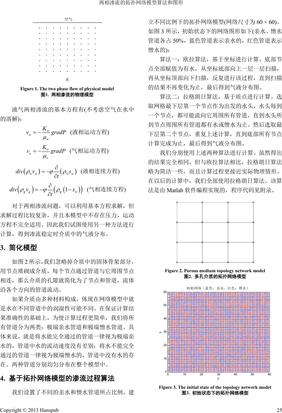 两相渗流的拓扑网络模型算法和图形 Copyright © 2013 Hanspub 25 空气 水 Figure 1. The two phase flow of physical model 图1. 两相渗流的物理模型 液气两相渗流的基本方程有(不考虑空气在水中 的溶解): w ww K vgradP (液相运动方程) o oo K vgradP (气相运动方程) ww ww div vs t (液相连续方程) 1 ggg w div vs t ( 气相连续方程) 对于两相渗流问题,可以利用基本方程求解,但 求解过程比较复杂,并且本模型中不存在压力,运动 方程不完全适用。因此我们试图使用另一种方法进行 计算,得到渗流稳定时介质中的气液分布。 3. 简化模型 如图 2所示,我们忽略掉介质中的固体骨架部分, 用节点堆砌成介质,每个节点通过管道与它周围节点 相连,那么介质的孔隙就简化为了节点和管道,流体 沿各个方向的管道流动。 如果介质由多种材料构成,体现在网络模型中就 是水在不同管道中的润湿性可能不同。在保证计算结 果准确性的基础上,为使计算过程更简单,我们将所 有管道分为两类:极端亲水管道和极端憎水管道。具 体来说,就是将水能完全通过的管道一律视为极端亲 水的,管道中水的流动速度没有差别;将水不能完全 通过的管道一律视为极端憎水的,管道中没有水的存 在。两种管道分别均匀分布在整个模型中。 4. 基于拓扑网络模型的渗流过程算法 我们设置了不同的亲水和憎水管道所占比例,建 立不同比例下的拓扑网络模型(网络尺寸为 60 × 60)。 如图 3所示,初始状态下的网络图形如下(亲水、憎水 管道各占 50%,蓝色管道表示亲水的,红色管道表示 憎水的): 算法一:欧拉算法,基于坐标进行计算。底部节 点全部赋值为有水,从坐标底部向上一层一层扫描, 再从坐标顶部向下扫描,反复进行该过程,直到扫描 的结果不再变化为止,最后得到气液分布图。 算法二:拉格朗日算法,基于质点进行计算。选 取网格最下层第一个节点作为出发的水头,水头每到 一个节点,都可能流向它周围所有管道,直到水头所 到节点周围所有管道都有水或憎水为止。然后选取最 下层第二个节点,重复上述计算,直到底部所有节点 计算完成为止,最后得到气液分布图。 我们分别使用上述两种算法进行计算。虽然得出 的结果完全相同,但与欧拉算法相比,拉格朗日算法 略为简洁一些,而且计算过程更接近实际物理情形。 在以后的计算中,我们全部使用拉格朗日算法。该算 法是由 Matlab 软件编程实现的,程序代码见附录。 Figure 2. Porous medium topology network model 图2. 多孔介质的拓扑网络模型 010 2030 4050 60 0 10 20 30 40 50 60 x y Figure 3. The initial state of the topology network model 图3. 初始状态下的拓扑网络模型 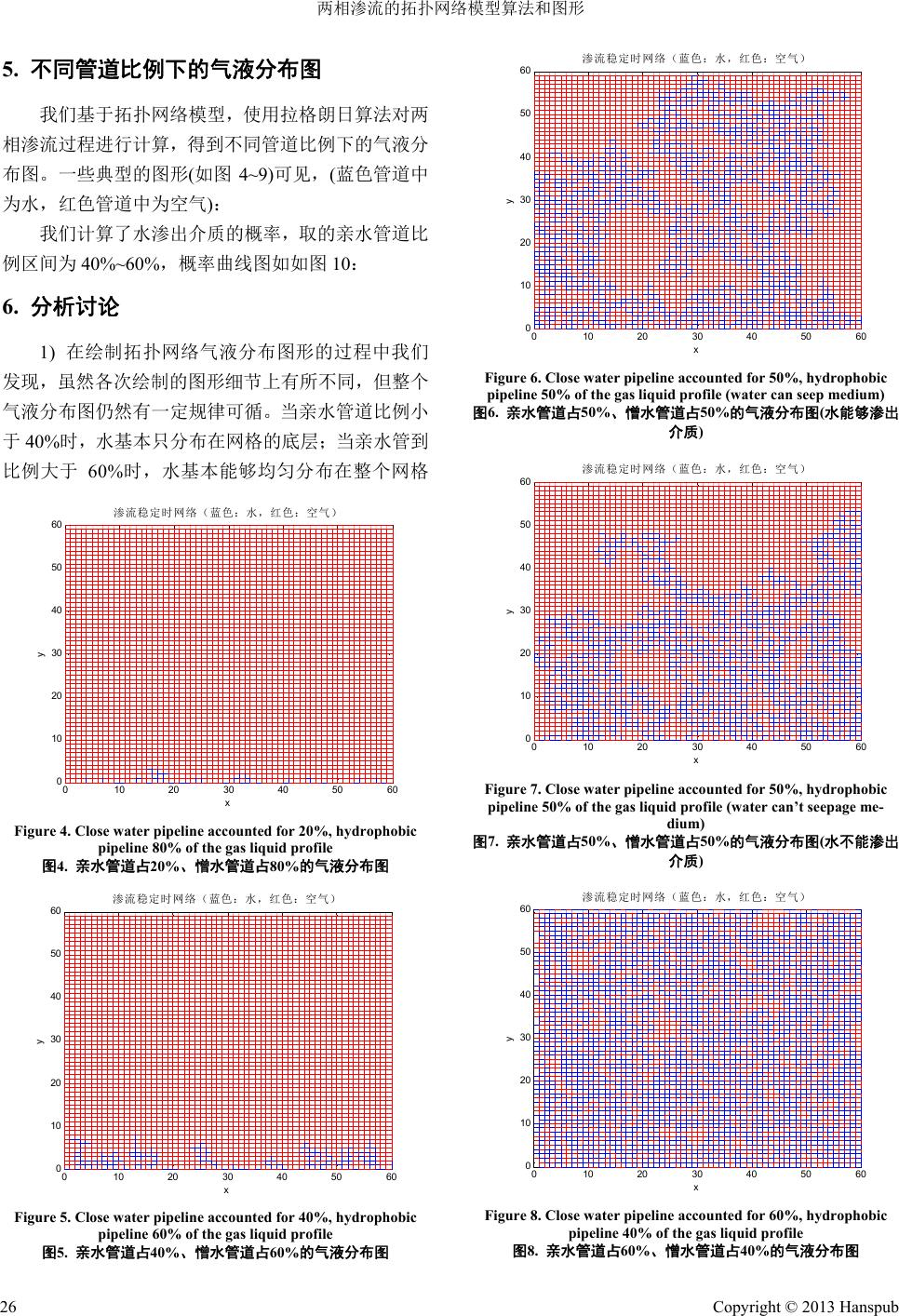 两相渗流的拓扑网络模型算法和图形 Copyright © 2013 Hanspub 26 5. 不同管道比例下的气液分布图 我们基于拓扑网络模型,使用拉格朗日算法对两 相渗流过程进行计算,得到不同管道比例下的气液分 布图。一些典型的图形(如图 4~9)可见,(蓝色管道中 为水,红色管道中为空气): 我们计算了水渗出介质的概率,取的亲水管道比 例区间为 40%~60%,概率曲线图如如图 10: 6. 分析讨论 1) 在绘制拓扑网络气液分布图形的过程中我们 发现,虽然各次绘制的图形细节上有所不同,但整个 气液分布图仍然有一定规律可循。当亲水管道比例小 于40%时,水基本只分布在网格的底层;当亲水管到 比例大于 60%时,水基本能够均匀分布在整个网格 010 2030 40 50 60 0 10 20 30 40 50 60 x y Figure 4. Close water pipeline accounted for 20%, hydrophobic pipeline 80% of the gas liquid profile 图4. 亲水管道占20%、憎水管道占80%的气液分布图 010 20 304050 60 0 10 20 30 40 50 60 x y Figure 5. Close water pipeline accounted for 40%, hydrophobic pipeline 60% of the gas liquid profile 图5. 亲水管道占40%、憎水管道占60%的气液分布图 010 20 30 40 5060 0 10 20 30 40 50 60 x y Figure 6. Close water pipeline accounted for 50%, hydrophobic pipeline 50% of the gas liquid profile (water can seep medium) 图6. 亲水管道占50%、憎水管道占50%的气液分布图(水能够渗出 介质) 010 20 30 40 5060 0 10 20 30 40 50 60 x y Figure 7. Close water pipeline accounted for 50%, hydrophobic pipeline 50% of the gas liquid profile (water can’t seepage me- dium) 图7. 亲水管道占50%、憎水管道占50%的气液分布图(水不能渗出 介质) 010 2030 40 5060 0 10 20 30 40 50 60 x y Figure 8. Close water pipeline accounted for 60%, hydrophobic pipeline 40% of the gas liquid profile 图8. 亲水管道占60%、憎水管道占40%的气液分布图  两相渗流的拓扑网络模型算法和图形 Copyright © 2013 Hanspub 27 010 2030 40 5060 0 10 20 30 40 50 60 x y Figure 9. Close water pipeline accounted for 80%, hydrophobic pipeline 20% of the gas liquid profile 图9. 亲水管道占80%、憎水管道占20%的气液分布图 0.40.42 0.440.46 0.480.50.52 0.540.56 0.580. 6 0 0.1 0.2 0.3 0.4 0.5 0.6 0.7 0.8 0.9 1 Figure 10. Chart water seepage probability curve 图10. 水渗出概率曲线 中。当亲水、憎水管到约各占一半时,会出现多种多 样的图形,有些图形中水较均匀地分布在网格的下半 部分,有些图形中水则较零散地分布在整个网格中。 2) 在亲水管道约占 50%的图形中,有些图形出现 了大面积的被水环绕的无水区域(如图 8),通常称之为 圈闭的死气区;还有一些图形的有水区域会沿着很细 的路径向上延伸(如图 9),通常称之为指进。 3) 从水渗出概率曲线(图10)中可以看出,当亲水 管道比例小于约 44%时,水基本无法渗出介质,当亲 水管道比例大于约 56%时,水一定能渗出介质,当亲 水管道比例处于 44%到56%之间时,水渗出介质是有 一定概率的,且概率随比例增大而增大。 7. 结论 本文将多孔介质简化为由节点和管道组成的拓 扑网络模型,并采用拉格朗日算法编程计算,绘制出 两相渗流情形下介质中气液分布的网络图,图形能够 表达更加细观的圈闭和指进等渗流图形,还可以由此 模型得出水渗出整个介质的概率。 参考文献 (References) [1] J. Bockris, S. Srinivasan. Fuel cell: Their electrochemistry. New York: McGraw-Hill Book Company, 1969: 230-253. [2] F. Huang. Three-dimensional reconstruction and simulation of porous media. University of Science and Technology of China, 2007: 5-122. [3] S. P. Guo, D. S. Yu and W. D. Wu. The physical characteristics of the porous media concerning flow in viscera. Acta Mechanica Sinica, 1982, (1): 29-36, 116-118. [4] X. Z. Xu, M. Zhu, F. Li and H. Song. Research on microstruc- ture of the gas diffusion electrode by the small pore diffusion law. Chinese Battery Industry, 2008, 13(1): 1-3. [5] B. M. Yu, P. Xu and J. Chen. Study on the seepage characteris- tics in fractured network porous media. Journal of Xi’an Shiyou University (Natural Science Edition), 2007, (2): 7-8, 37-38, 41. [6] P. Chen, C. F. Wei, J. L. Wang, P. P. Yi and H. F. Cao. Numerical analysis of seepage processes in unsaturated porous media under nearly saturated conditions. Rock and Soil Mechanics, 2012, (1): 299-304.  两相渗流的拓扑网络模型算法和图形 Copyright © 2013 Hanspub 28 附录:主要计算程序代码 M = 61;N = 60; A = rand(M,N);B = rand(N,M) ;P = zeros(M); Z = zeros(1,2*M*M);top = −1; p = input(''); for j = 1:M P(1,j) = 1; end for j = 1:M*N if A(j) < p A(j) = 1; else A(j) = 0; end if B(j) < p B(j) = 1; else B(j) = 0; end end for k = 1:M top = top + 2; Z(top) = 1;Z(top + 1) = k; for j = 1:M*M if Z(top) < M&&B(Z(top),Z(top + 1)) = 1&&P(Z(top) + 1,Z(top + 1)) = 0 Z(top + 2) = Z(top) + 1; Z(top + 3) = Z(top + 1); top = top + 2; P(Z(top),Z(top + 1)) = 1; elseif Z(top + 1) < M&&A(Z(top),Z(top + 1)) = 1&&P (Z(top),Z(top + 1) + 1) = 0 Z(top + 2) = Z(top); Z(top + 3) = Z(top + 1) + 1; top = top + 2; P(Z(top),Z(top + 1)) = 1; elseif Z(top) > 1&&B(Z(top)-1,Z(top + 1)) = 1&&P(Z(top)-1,Z(top + 1)) = = 0 Z(top + 2) = Z(top) − 1; Z(top + 3) = Z(top + 1); top = top + 2; P(Z(top),Z(top + 1)) = 1; elseif Z(top + 1) > 1&&A(Z(top),Z(top + 1)−1) = 1&&P(Z(top),Z(top + 1) − 1) = 0 Z(top + 2) = Z(top); Z(top + 3) = Z(top + 1) − 1; top = top + 2; P(Z(top),Z(top + 1)) = 1; else top = top − 2; end end end end if top = −1 break; end end end for m = 1:M for n = 1:N if P(m,n) = 0&&P(m,n + 1) = 0 A(m,n) = 0; end if P(n,m) = 0&&P(n + 1,m) = 0 B(n,m) = 0; end end end for m = 1:M for n = 1:N x = n−1:n; if A(m,n) = 1 plot(x,x*0 + m − 1); else plot(x,x*0 + m − 1,'r'); end holdon; if B(n,m) = 1 plot(x*0 + m − 1,x); else plot(x*0 + m − 1,x,'r'); end holdon; end end |